Forecasting Tuna Fisheries

This project was part of a statistics course in environmental econometrics. My task was to develop a robust model to predict trends in environmental data, as well as write a paper that critically analyses the findings and offers potential contributing factors.

The best resource I found that helped me understand the process of this analysis was in an online book (Gijón Air Pollution - An exercise of visualization and forecasting). Check out chapter 8 for ARIMA models! (https://bookdown.org/sergioberdiales/tfm-kschool_gijon_air_pollution/forecasting-models-arima.html)

Dataset retrieved from TCASHION on Kaggle (https://www.kaggle.com/datasets/tcashion/tokyo-wholesale-tuna-prices/code)

The Tsukiji fish market, which operated until 2018, was the largest wholesale fish market in the world, specializing in sashimi tunas.

Species Covered:

• Bluefin Tuna

• Southern Bluefin Tuna

• Bigeye Tuna

Measures

• Quantity - Metric tonnes (i.e, 1000 kilograms)

• Price - Yen / kilogram

1. Install and Load Packages

options(repos = c(CRAN = "https://cloud.r-project.org"))
library(fpp2)

Registered S3 method overwritten by 'quantmod':
  method            from
  as.zoo.data.frame zoo 

── Attaching packages ────────────────────────────────────────────── fpp2 2.5 ──

✔ ggplot2   3.5.1      ✔ fma       2.5   
✔ forecast  8.22.0     ✔ expsmooth 2.3   

library(TTR)
library(forecast)
library(tseries)
library(lubridate)

Attaching package: 'lubridate'

The following objects are masked from 'package:base':

    date, intersect, setdiff, union

library(tidyverse)

── Attaching core tidyverse packages ──────────────────────── tidyverse 2.0.0 ──
✔ dplyr   1.1.4     ✔ stringr 1.5.1
✔ forcats 1.0.0     ✔ tibble  3.2.1
✔ purrr   1.0.2     ✔ tidyr   1.3.1
✔ readr   2.1.5     

── Conflicts ────────────────────────────────────────── tidyverse_conflicts() ──
✖ dplyr::filter() masks stats::filter()
✖ dplyr::lag()    masks stats::lag()
ℹ Use the conflicted package (<http://conflicted.r-lib.org/>) to force all conflicts to become errors

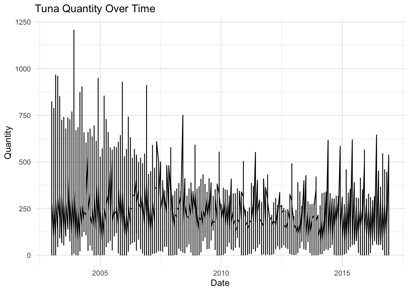
2. Plot Quantity and Price

tuna<-read.csv("/Users/owencallahan/Desktop/R/tokyo_wholesale_tuna_prices.csv")

# Combine month and year collumn
tuna <- tuna %>%
  mutate(date = make_date(year, month))

# Sort data by date
tuna <- tuna %>% arrange(date)

# Plot Quantity
tuna_quantity <- tuna %>%
  filter(measure == "Quantity")

ggplot(tuna_quantity, aes(x = date, y = value)) +
  geom_line() +
  labs(title = "Tuna Quantity Over Time", x = "Date", y = "Quantity") +
  theme_minimal()

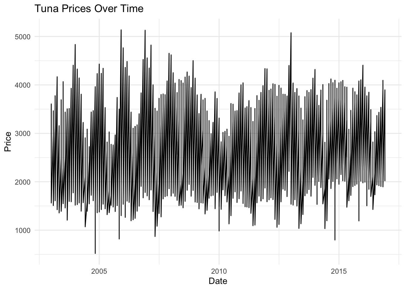
# Plot Price
tuna_price <- tuna %>%
  filter(measure == "Price")

ggplot(tuna_price, aes(x = date, y = value)) +
  geom_line() +
  labs(title = "Tuna Prices Over Time", x = "Date", y = "Price") +
  theme_minimal()

3. Model Selection

• Trend: Look for any long-term movements or patterns in the data.

• Seasonality: Check for repeating patterns at fixed intervals

• Randomness: Assess if there are irregular fluctuations or noise.

Decomposition: helps in separating a time series into its components:

• When to Use:

  • If there is a clear trend and/or seasonal pattern in the data, decomposition can help isolate these components for better analysis and forecasting.

Moving Average Smoothing: is used to reduce short-term fluctuations in the data:

• When to Use:

  • To smooth out irregular fluctuations or noise in the data, making underlying patterns more apparent.

Exponential Smoothing: assigns exponentially decreasing weights to older observations:

• When to Use:

  • When the data has no clear trend or seasonality but exhibits random fluctuations.

  • For short-term forecasting where recent data points are more relevant.

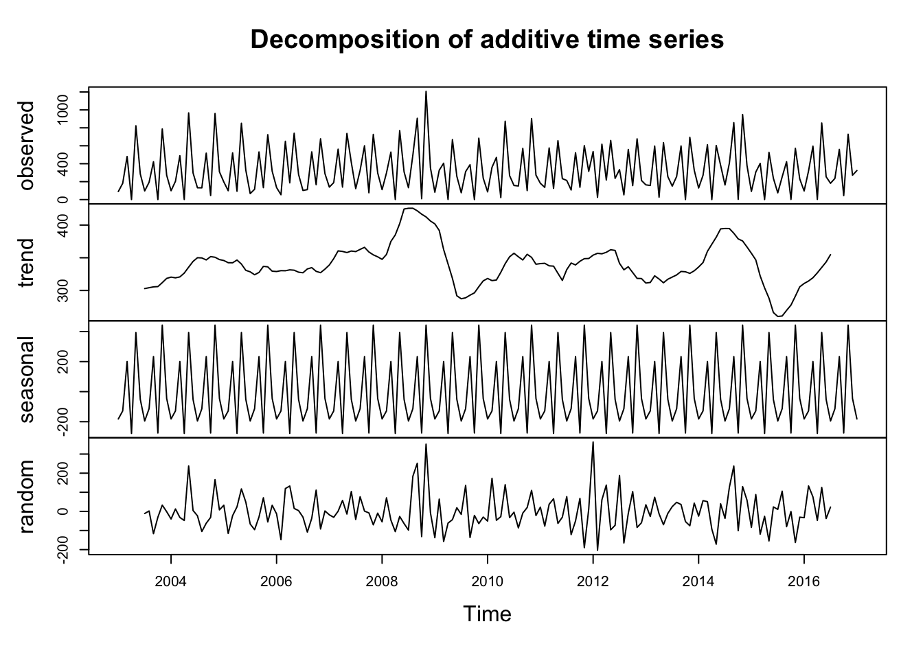
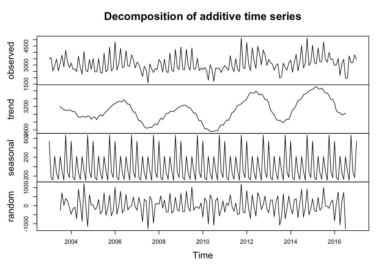
# Quantity
ts_quan <- ts(tuna_quantity$value, start = 2003, end = 2017,frequency = 12)  
decomposed1 <- decompose(ts_quan)
plot(decomposed1)

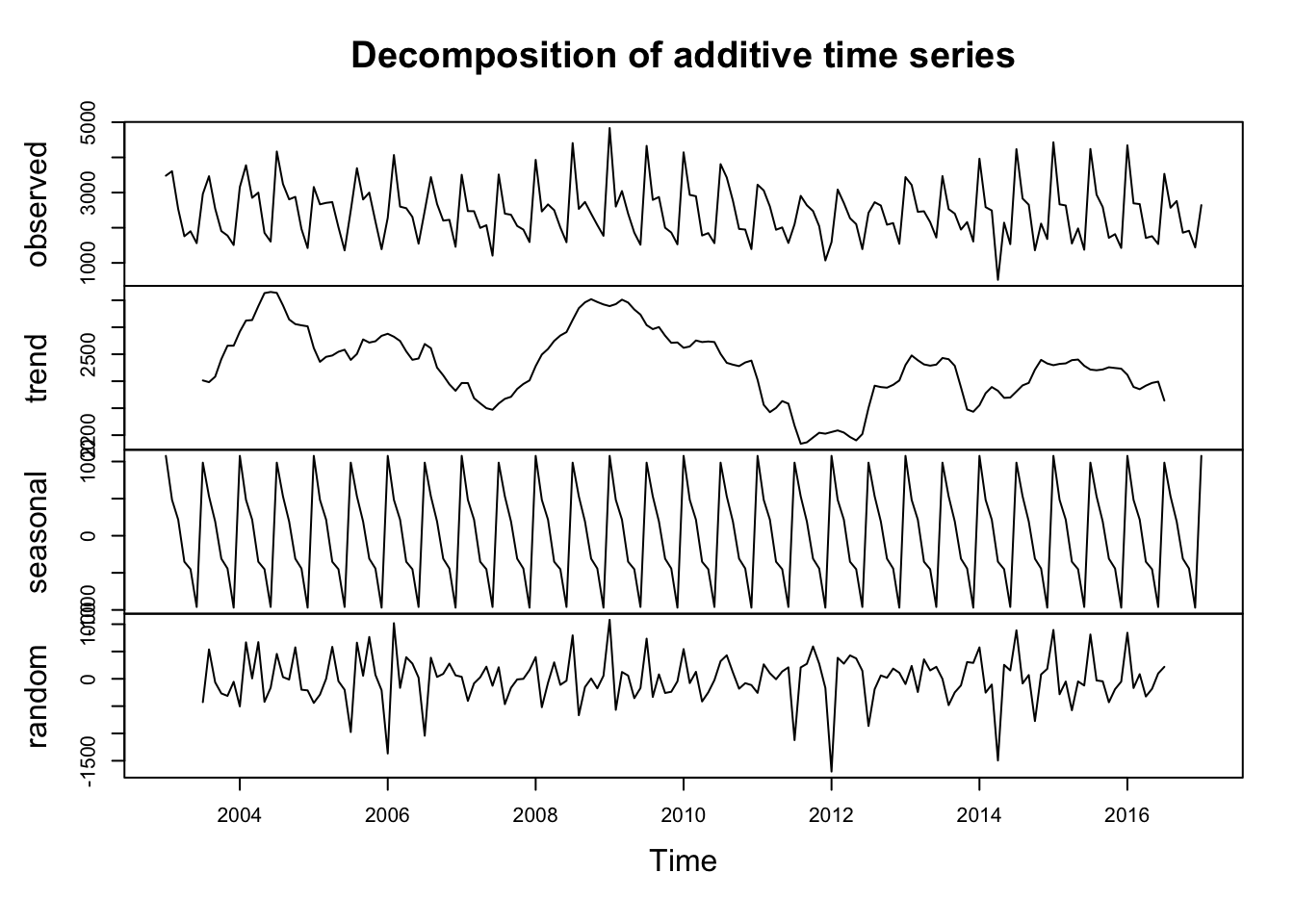
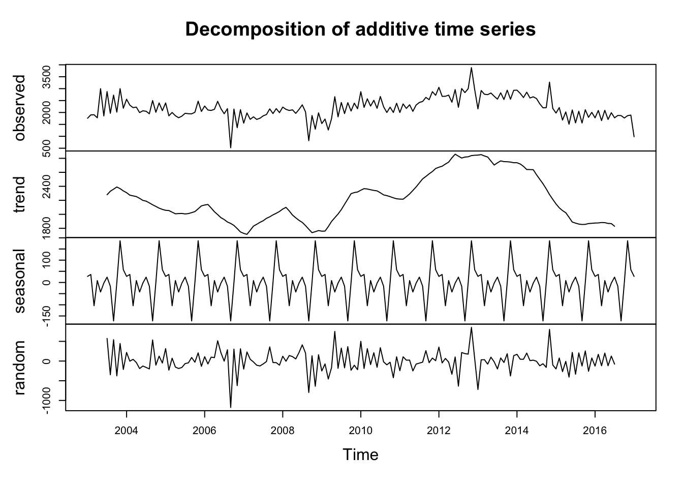
# Price
ts_price <- ts(tuna_price$value, start = 2003, end = 2017, frequency = 12)  
decomposed2 <- decompose(ts_price)
plot(decomposed2) 

Key Takeaways

• Seasonal Component: Appears consistent, suggesting recurring patterns at regular intervals.

• Trend Component: Appears less predictable, indicating potential long-term shifts or fluctuations that are not easily captured by a simple pattern.

• Random Component: Shows variability, indicating unexplained fluctuations or noise in the data.

4. Test for Stationarity

The ADF test is a statistical test that assesses whether a time series is stationary. Stationarity means that the statistical properties of a time series (such as mean, variance, and autocorrelation) do not change over time.

• A more negative ADF statistic indicates stronger evidence for stationarity.

# ADF test
adf_test <- adf.test(ts_price)
print(adf_test)

    Augmented Dickey-Fuller Test

data:  ts_price
Dickey-Fuller = -2.7664, Lag order = 5, p-value = 0.2563
alternative hypothesis: stationary

adf_test <- adf.test(ts_quan)
print(adf_test)

    Augmented Dickey-Fuller Test

data:  ts_quan
Dickey-Fuller = -3.0099, Lag order = 5, p-value = 0.1547
alternative hypothesis: stationary

Key Takeaways

• Price model is not stationary

• Quantity model is not stationary

5. Fit an ARIMA model

# Fit model
fit_price <- auto.arima(ts_price)
fit_quan <- auto.arima(ts_quan)

# Summary
summary(fit_price)

Series: ts_price 
ARIMA(0,0,0)(0,1,1)[12] with drift 

Coefficients:
         sma1    drift
      -0.8494  -1.3377
s.e.   0.0865   0.8690

sigma^2 = 235806:  log likelihood = -1200.48
AIC=2406.96   AICc=2407.12   BIC=2416.13

Training set error measures:
                   ME     RMSE      MAE       MPE     MAPE     MASE        ACF1
Training set 12.06902 465.0506 303.0941 -3.201486 13.59532 0.840122 -0.05292377

summary(fit_quan)

Series: ts_quan 
ARIMA(0,0,0)(1,1,0)[12] with drift 

Coefficients:
         sar1   drift
      -0.4004  0.1308
s.e.   0.0729  0.6294

sigma^2 = 16957:  log likelihood = -987.28
AIC=1980.57   AICc=1980.72   BIC=1989.73

Training set error measures:
                    ME     RMSE      MAE      MPE     MAPE      MASE
Training set 0.9639297 124.7093 87.62616 -578.987 607.8686 0.9004508
                    ACF1
Training set -0.01891516

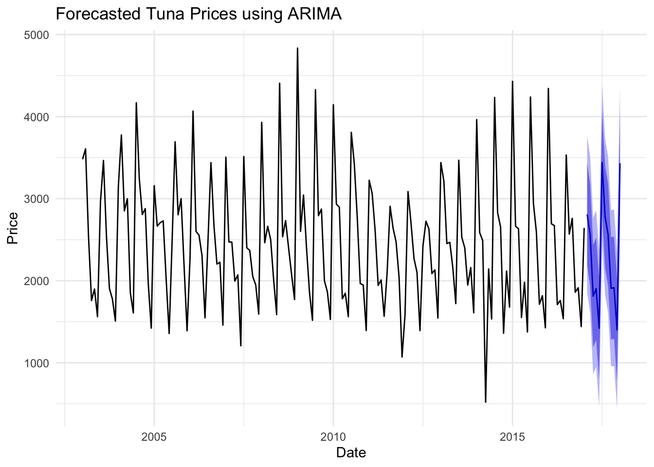
# Forecasting Price
fore_price <- forecast(fit_price, h = 12)
autoplot(fore_price) +
  labs(title = "Forecasted Tuna Prices using ARIMA", x = "Date", y = "Price") +
  theme_minimal()

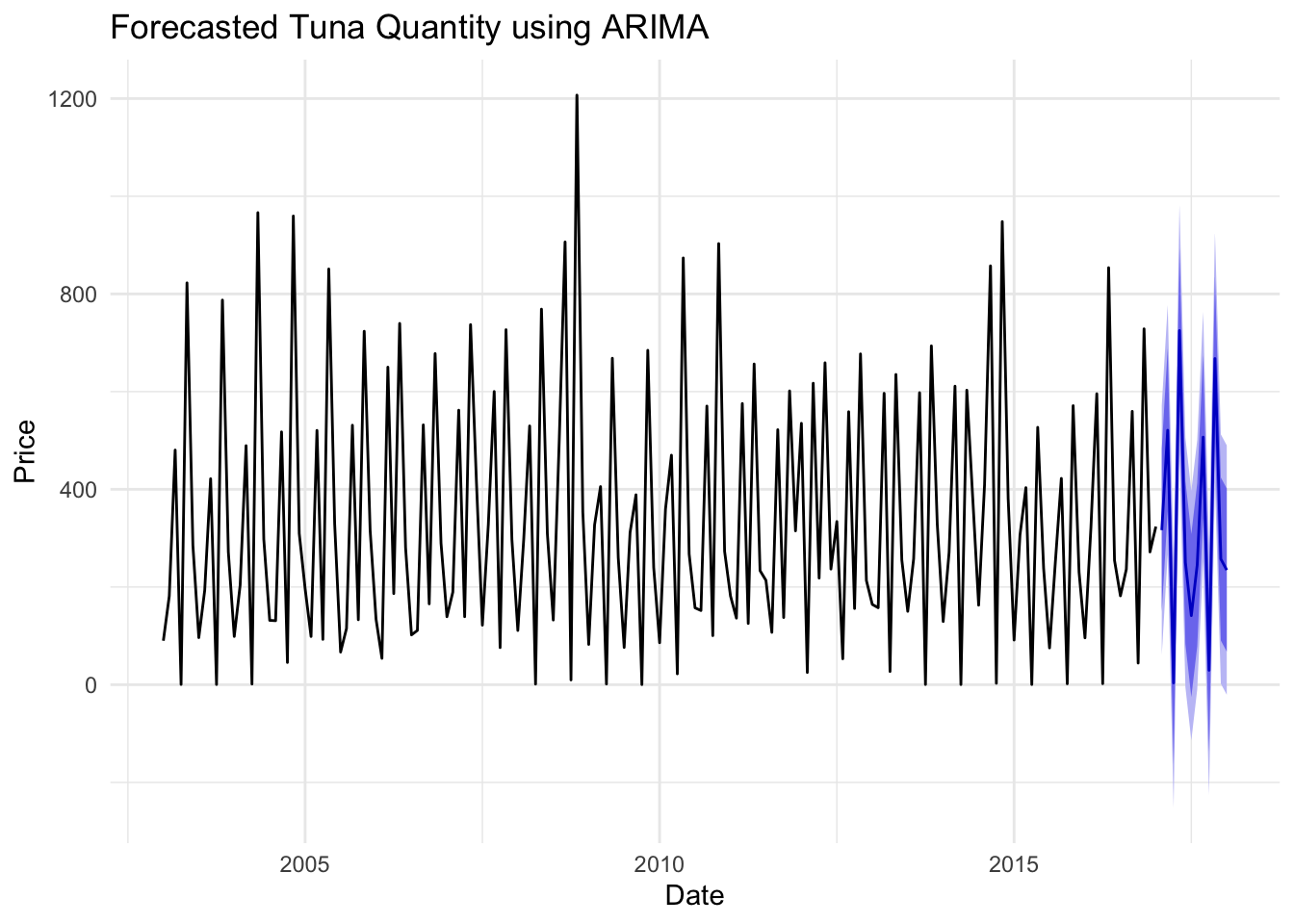
# Forecasting Quantity
fore_quan <- forecast(fit_quan, h = 12) 
autoplot(fore_quan) +
  labs(title = "Forecasted Tuna Quantity using ARIMA", x = "Date", y = "Price") +
  theme_minimal()

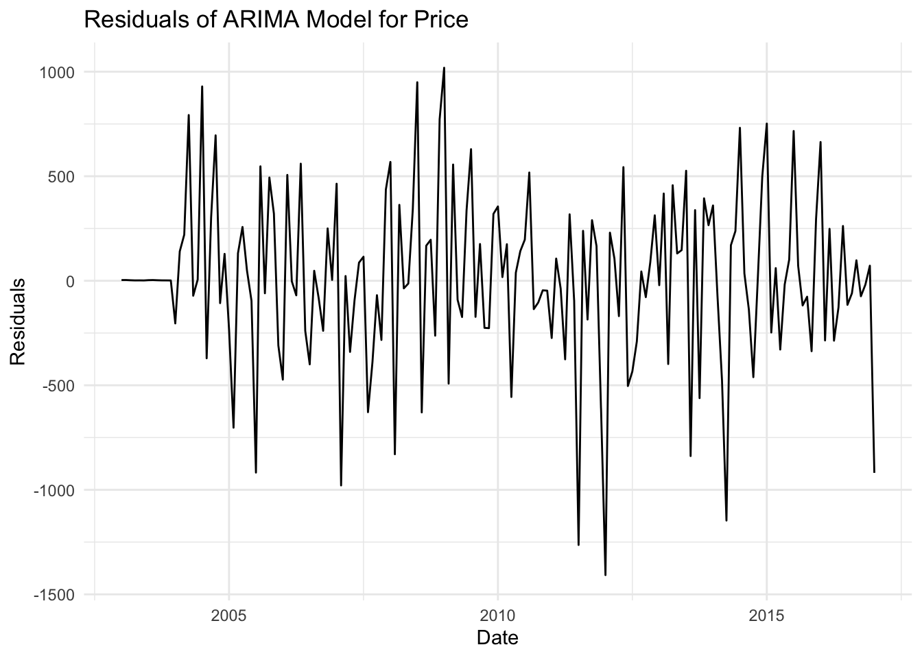
6. Evaluate Results

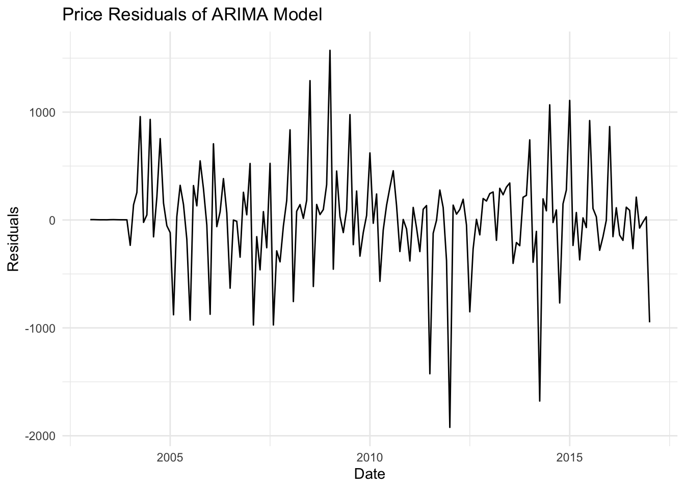
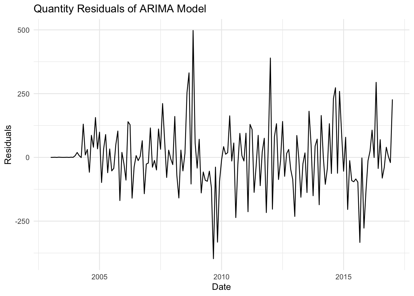
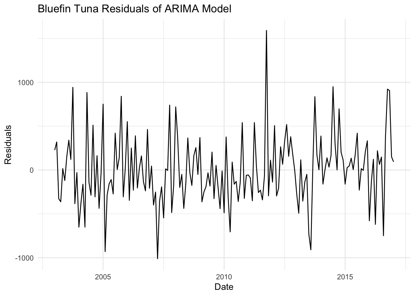
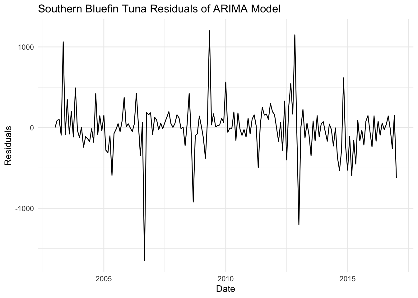
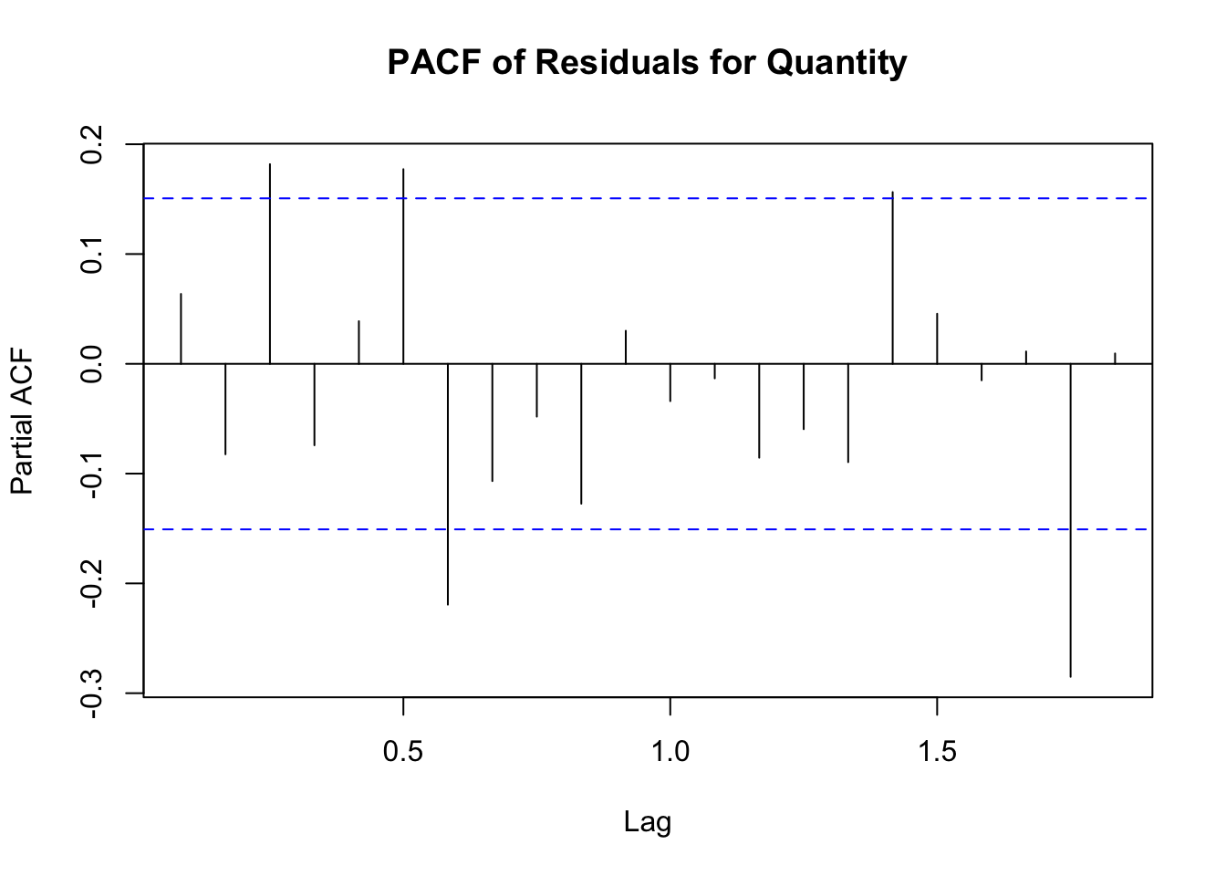
• Residual Plot: Inspect the plot to ensure the residuals are centered around zero and exhibit constant variance. If there are patterns or trends in the residuals, it suggests that the model may need improvement.

• Mean Squared Error (MSE): A smaller MSE indicates that the model’s predictions are closer to the actual values, implying better model performance.

# Residuals
residuals_p <- residuals(fit_price)
residuals_q <- residuals(fit_quan)

# Plot residuals
autoplot(residuals_p) + 
  labs(title = "Price Residuals of ARIMA Model", x = "Date", y = "Residuals") +
  theme_minimal()

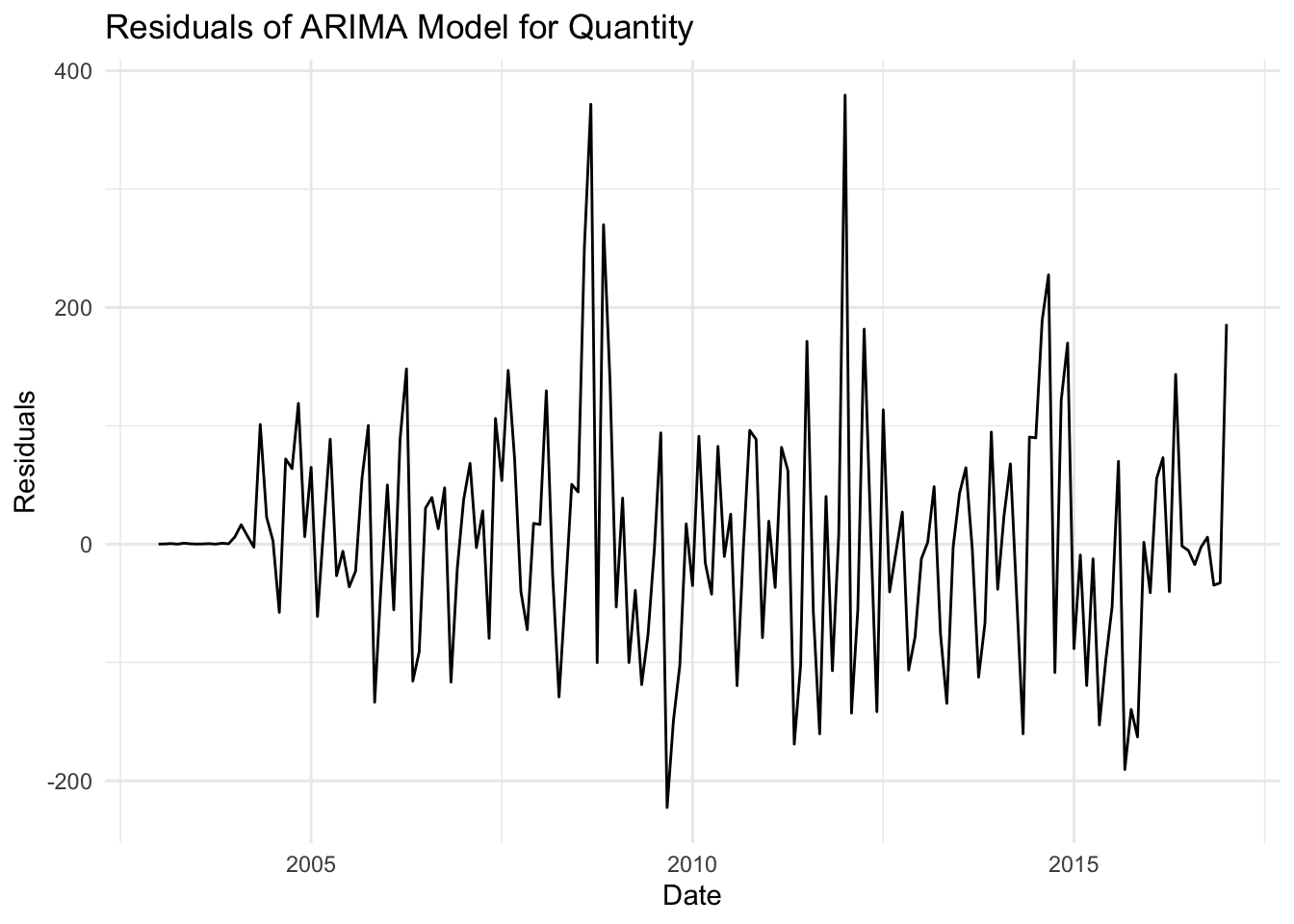
autoplot(residuals_q) + 
  labs(title = "Quantity Residuals of ARIMA Model", x = "Date", y = "Residuals") +
  theme_minimal()

# Calculate performance metrics
MSE_p <- mean(residuals_p^2)
RMSE_p <- sqrt(MSE_p)
MAE_p <- mean(abs(residuals_p))

MSE_q <- mean(residuals_q^2)
RMSE_q <- sqrt(MSE_q)
MAE_q <- mean(abs(residuals_q))

# R-squared
SS_total <- sum((ts_price - mean(ts_price))^2)
SS_residual <- sum(residuals_p^2)
R_squared_p <- 1 - (SS_residual / SS_total)

SS_total_q <- sum((ts_quan - mean(ts_quan))^2)
SS_residual_q <- sum(residuals_q^2)
R_squared_q <- 1 - (SS_residual_q / SS_total_q)

cat("MSE:", MSE_p, "\n")

MSE: 216272.1 

cat("RMSE:", RMSE_p, "\n")

RMSE: 465.0506 

cat("MAE:", MAE_p, "\n")

MAE: 303.0941 

cat("R-squared:", R_squared_p, "\n")

R-squared: 0.6573022 

cat("MSE:", MSE_q, "\n")

MSE: 15552.41 

cat("RMSE:", RMSE_q, "\n")

RMSE: 124.7093 

cat("MAE:", MAE_q, "\n")

MAE: 87.62616 

cat("R-squared:", R_squared_q, "\n")

R-squared: 0.7745865 

Key Takeaways

• Price Model:

  • The price model shows moderate explanatory power (R² = 0.657), but the high MSE and RMSE indicate that the residuals are substantial, suggesting potential improvements or alternative modeling techniques might be needed.

• Quantity Model:

  • The quantity model shows better performance with higher R² (0.775) and lower error metrics (MSE, RMSE, MAE), indicating a good fit and more accurate predictions compared to the price model.

7. Exploratory Data Analysis with Different Species

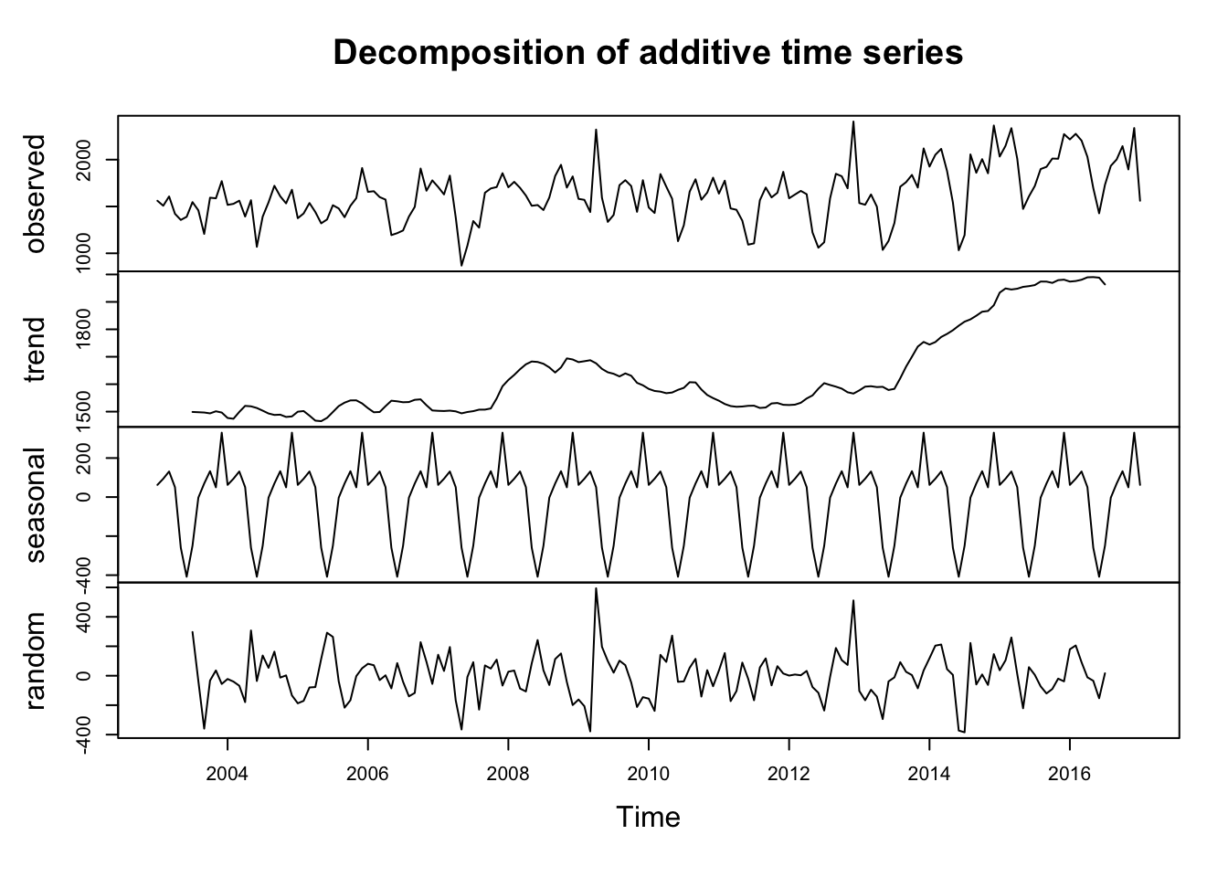
bt_price <- tuna %>%
  filter(measure == "Price",
         species == "Bluefin Tuna")
ts_bt <- ts(bt_price$value, start = 2003, end = 2017, frequency = 12)  
decomposed3 <- decompose(ts_bt)
plot(decomposed3) 

sbt_price <- tuna %>%
  filter(measure == "Price",
         species == "Southern Bluefin Tuna")
ts_sbt <- ts(sbt_price$value, start = 2003, end = 2017, frequency = 12)  
decomposed4 <- decompose(ts_sbt)
plot(decomposed4) 

bgt_price <- tuna %>%
  filter(measure == "Price",
         species == "Bigeye Tuna")
ts_bgt <- ts(bgt_price$value, start = 2003, end = 2017, frequency = 12)  
decomposed5 <- decompose(ts_bgt)
plot(decomposed5) 

Key Takeaways

• Seasonal Component: Appears consistent, suggesting recurring patterns at regular intervals.

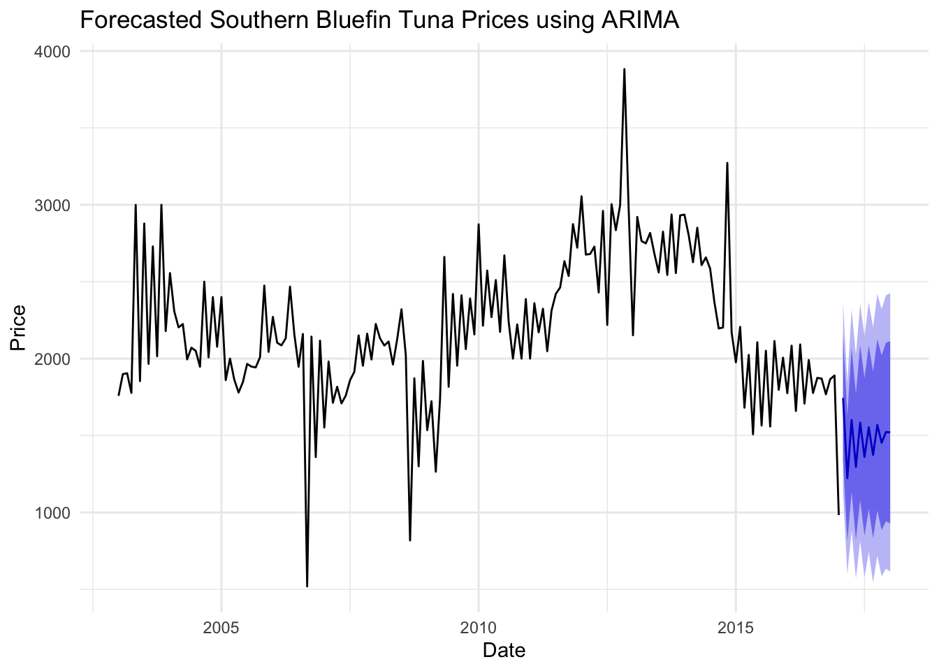
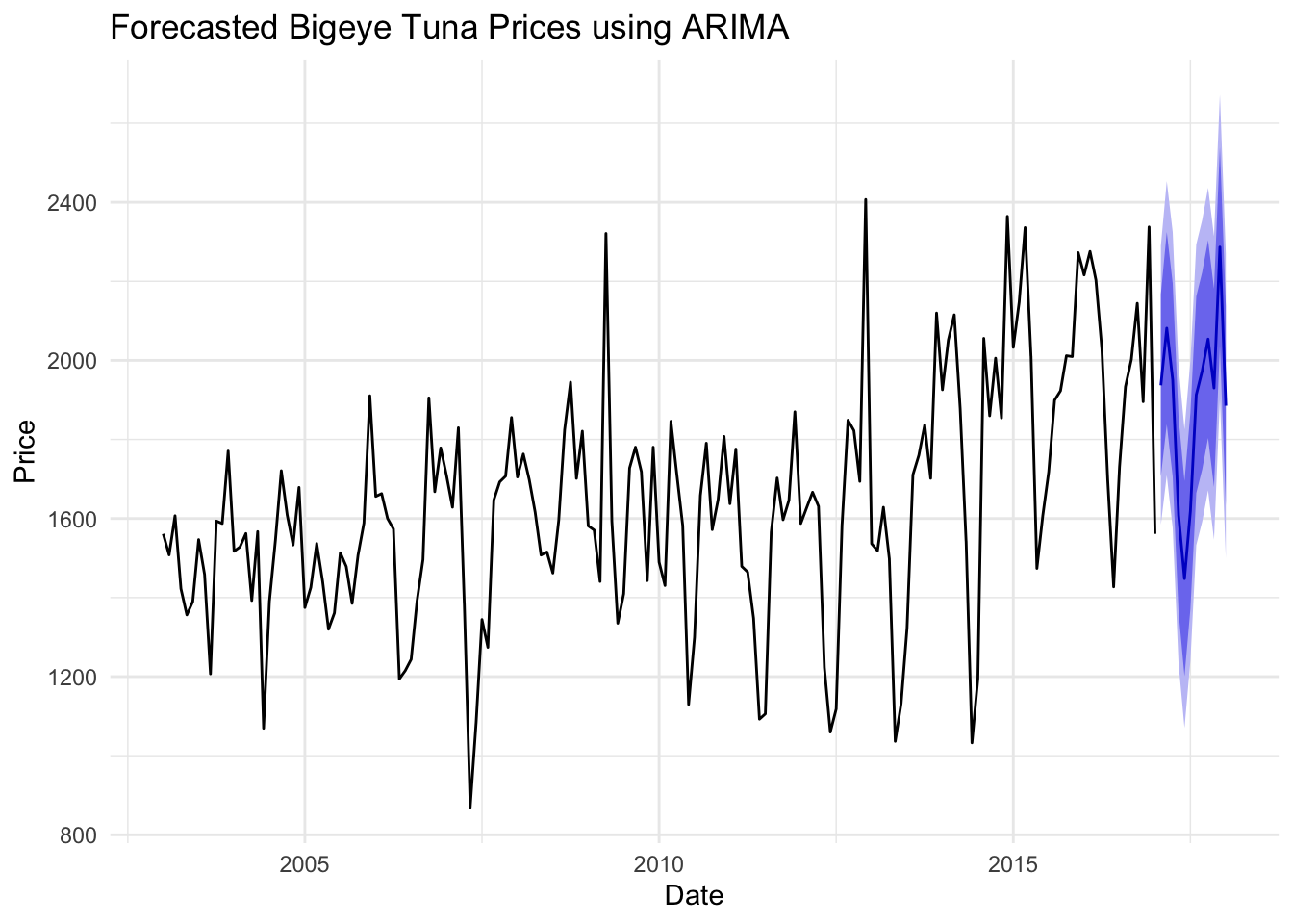
• Trend Component: Bluefin Tuna has a predictable trend, however Southern Bluefin and Bigeye Tuna appears less predictable, both indicating potential long-term jump in price over time.

• Random Component: Shows variability, indicating unexplained fluctuations or noise in the data.

# Quickly check for stationarity
adf.test(ts_bt)

Warning in adf.test(ts_bt): p-value smaller than printed p-value

    Augmented Dickey-Fuller Test

data:  ts_bt
Dickey-Fuller = -4.0301, Lag order = 5, p-value = 0.01
alternative hypothesis: stationary

adf.test(ts_sbt)

    Augmented Dickey-Fuller Test

data:  ts_sbt
Dickey-Fuller = -1.5708, Lag order = 5, p-value = 0.7555
alternative hypothesis: stationary

adf.test(ts_bgt)

Warning in adf.test(ts_bgt): p-value smaller than printed p-value

    Augmented Dickey-Fuller Test

data:  ts_bgt
Dickey-Fuller = -6.438, Lag order = 5, p-value = 0.01
alternative hypothesis: stationary

Key Takeaways

• Bluefin Tuna: Stationary

• Southern Bluefin: Non-Stationary

• Bigeye Tuna: Stationary

# Fit model
fit_bt <- auto.arima(ts_bt)
fit_sbt <- auto.arima(ts_sbt)
fit_bgt <- auto.arima(ts_bgt)

summary(fit_bt)

Series: ts_bt 
ARIMA(4,0,0)(2,0,1)[12] with non-zero mean 

Coefficients:
         ar1      ar2     ar3      ar4     sar1     sar2    sma1       mean
      0.0691  -0.0463  0.7589  -0.1061  -0.7768  -0.3637  0.7588  3114.3466
s.e.  0.0788   0.0502  0.0496   0.0795   0.1202   0.0820  0.1127    75.9551

sigma^2 = 162826:  log likelihood = -1254.42
AIC=2526.83   AICc=2527.96   BIC=2555

Training set error measures:
                   ME     RMSE      MAE       MPE     MAPE      MASE
Training set 2.517485 393.8503 296.0585 -1.518045 9.976024 0.4364676
                    ACF1
Training set 0.002743469

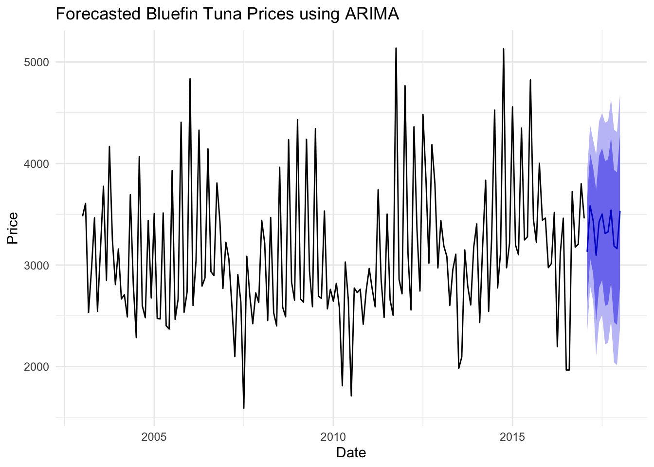
# Forecasting Different Specices
fore_price3 <- forecast(fit_bt, h = 12) 
autoplot(fore_price3) +
  labs(title = "Forecasted Bluefin Tuna Prices using ARIMA", x = "Date", y = "Price") +
  theme_minimal()

fore_price4 <- forecast(fit_sbt, h = 12) 
autoplot(fore_price4) +
  labs(title = "Forecasted Southern Bluefin Tuna Prices using ARIMA", x = "Date", y = "Price") +
  theme_minimal()

fore_price5 <- forecast(fit_bgt, h = 12)
autoplot(fore_price5) +
  labs(title = "Forecasted Bigeye Tuna Prices using ARIMA", x = "Date", y = "Price") +
  theme_minimal()

# Residuals
residuals_1 <- residuals(fit_bt)
residuals_2 <- residuals(fit_sbt)
residuals_3 <- residuals(fit_bgt)

# Plot residuals
autoplot(residuals_1) + 
  labs(title = "Bluefin Tuna Residuals of ARIMA Model", x = "Date", y = "Residuals") +
  theme_minimal()

autoplot(residuals_2) + 
  labs(title = "Southern Bluefin Tuna Residuals of ARIMA Model", x = "Date", y = "Residuals") +
  theme_minimal()

autoplot(residuals_3) + 
  labs(title = "Bigeye Tuna Residuals of ARIMA Model", x = "Date", y = "Residuals") +
  theme_minimal()

8. Model Improvement

# Price model
fit_price1 <- auto.arima(ts_price, stepwise = FALSE, approximation = FALSE)

# Quantity model
fit_quantity1 <- auto.arima(ts_quan, stepwise = FALSE, approximation = FALSE)

# Generate forecasts and calculate residuals again
fore_price <- forecast(fit_price1, h = 12)
residuals_p1 <- residuals(fit_price1)

fore_quantity <- forecast(fit_quantity1, h = 12)
residuals_q1 <- residuals(fit_quantity1)

# Performance metrics
MSE_p1 <- mean(residuals_p1^2)
RMSE_p1 <- sqrt(MSE_p1)
MAE_p1 <- mean(abs(residuals_p1))
SS_total_p1 <- sum((ts_price - mean(ts_price))^2)
SS_residual_p1 <- sum(residuals_p1^2)
R_squared_p1 <- 1 - (SS_residual_p1 / SS_total_p1)

MSE_q1 <- mean(residuals_q1^2)
RMSE_q1 <- sqrt(MSE_q1)
MAE_q1 <- mean(abs(residuals_q1))
SS_total_q1 <- sum((ts_quan - mean(ts_quan))^2)
SS_residual_q1 <- sum(residuals_q1^2)
R_squared_q1 <- 1 - (SS_residual_q1 / SS_total_q1)

cat("Updated Metrics for Price Model\n")

Updated Metrics for Price Model

cat("MSE:", MSE_p1, "\n")

MSE: 165858.2 

cat("RMSE:", RMSE_p1, "\n")

RMSE: 407.2569 

cat("MAE:", MAE_p1, "\n")

MAE: 296.6826 

cat("R-squared:", R_squared_p1, "\n")

R-squared: 0.7371865 

cat("Updated Metrics for Quantity Model\n")

Updated Metrics for Quantity Model

cat("MSE:", MSE_q1, "\n")

MSE: 9458.524 

cat("RMSE:", RMSE_q1, "\n")

RMSE: 97.25494 

cat("MAE:", MAE_q1, "\n")

MAE: 70.89373 

cat("R-squared:", R_squared_q1, "\n")

R-squared: 0.86291 

9. Diagnostics

# Plot residuals
autoplot(residuals_p1) + 
  labs(title = "Residuals of ARIMA Model for Price", x = "Date", y = "Residuals") +
  theme_minimal()

autoplot(residuals_q1) + 
  labs(title = "Residuals of ARIMA Model for Quantity", x = "Date", y = "Residuals") +
  theme_minimal()

# ACF and PACF of residuals
acf(residuals_p1, main="ACF of Residuals for Price")

pacf(residuals_p1, main="PACF of Residuals for Price")

acf(residuals_q1, main="ACF of Residuals for Quantity")

pacf(residuals_q1, main="PACF of Residuals for Quantity")

# Ljung-Box test for autocorrelation
Box.test(residuals_p1, lag = 20, type = "Ljung-Box")

    Box-Ljung test

data:  residuals_p1
X-squared = 91.573, df = 20, p-value = 3.93e-11

Box.test(residuals_q1, lag = 20, type = "Ljung-Box")

    Box-Ljung test

data:  residuals_q1
X-squared = 48.397, df = 20, p-value = 0.0003741

In this analysis, I aimed to model and forecast tuna prices and quantities using ARIMA models. After refining the models, there were significant improvements in the performance metrics for both the price and quantity models.

The updated price model shows a substantial reduction in error metrics and an increase in explanatory power, with the R-squared value improving from 0.657 to 0.737. This indicates that the model now explains approximately 73.72% of the variance in the price data, suggesting a more accurate and reliable model.

The quantity model also shows improved performance, with lower error metrics and a higher R-squared value, now at 0.86291. This indicates that the model explains about 86.29% of the variance in the quantity data.

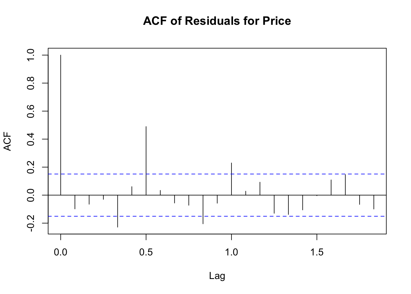
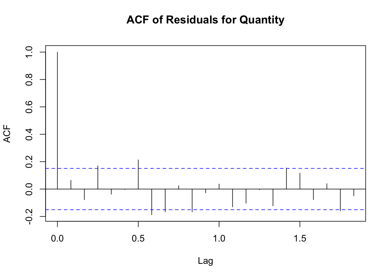
The p-values for both tests are significantly lower than 0.05, indicating that there is still some autocorrelation in the residuals, suggesting that the models could be further refined. However, the current models still provide a substantial improvement over the initial attempts.