Considering my love for exercise and health, I found a dataset on physical activity and heart rate to use for a Bayesian analysis. I am interested in exploring the relationship between exercise and heart rate, which calls for a linear regression approach. To perform a Bayesian linear regression, I will use the brms package in R. This package provides an interface to fit complex Bayesian models using the probabilistic programming language Stan. Stan’s efficient Hamiltonian Monte Carlo algorithms can sample from the posterior distribution of the model parameters.
I could not have learned some of these steps by myself. An amazing resource to check out is bayesrulesbook.com; it will teach you so much about the Bayesian philosophy and techniques. If you curious about where I learned some of the steps below, check out Chapter 6!
Loading 'brms' package (version 2.21.0). Useful instructions
can be found by typing help('brms'). A more detailed introduction
to the package is available through vignette('brms_overview').
Attaching package: 'brms'
The following object is masked from 'package:stats':

    ar
library(bayesplot)
This is bayesplot version 1.11.1
- Online documentation and vignettes at mc-stan.org/bayesplot
- bayesplot theme set to bayesplot::theme_default()
* Does _not_ affect other ggplot2 plots
* See ?bayesplot_theme_set for details on theme setting
Attaching package: 'bayesplot'
The following object is masked from 'package:brms':

    rhat
# We can model heart rate as a function of physical activity, age, weight, and gendermodel <-brm( heart_rate ~ physical_activity + age + weight + gender,data = data,family =gaussian(),prior =c(set_prior("normal(0, 10)", class ="b")) # set a normal prior of M = 0 and SD = 10)
# Print a summary of the fitted model, we can assess our estimates and our credible intervalssummary(model)
 Family: gaussian
  Links: mu = identity; sigma = identity
Formula: heart_rate ~ physical_activity + age + weight + gender
   Data: data (Number of observations: 145)
  Draws: 4 chains, each with iter = 2000; warmup = 1000; thin = 1;
         total post-warmup draws = 4000

Regression Coefficients:
                  Estimate Est.Error l-95% CI u-95% CI Rhat Bulk_ESS Tail_ESS
Intercept            75.58      9.77    56.75    94.34 1.00     6425     3275
physical_activity    -0.06      0.12    -0.29     0.17 1.00     5619     3328
age                   0.05      0.05    -0.04     0.14 1.00     5681     2843
weight                0.01      0.10    -0.18     0.20 1.00     6231     3241
genderMale           -0.83      1.72    -4.14     2.51 1.00     5424     3195

Further Distributional Parameters:
      Estimate Est.Error l-95% CI u-95% CI Rhat Bulk_ESS Tail_ESS
sigma    10.68      0.63     9.52    12.03 1.00     4866     2718

Draws were sampled using sampling(NUTS). For each parameter, Bulk_ESS
and Tail_ESS are effective sample size measures, and Rhat is the potential
scale reduction factor on split chains (at convergence, Rhat = 1).
Important Note: Credible intervals crossing through 0 in Bayesian analysis indicate uncertainty or lack of evidence for a nonzero effect. Also, a replication of this study may reveal different conclusions.
3. Data Visualization
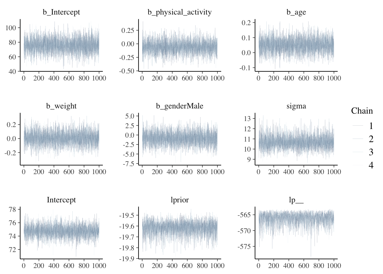
Trace Plots: Displays the sampled values of the parameters over iterations of the Markov Chain Monte Carlo sampling.
Interpretation: Look for a fuzzy caterpillar where the chains mix well and cover the parameter space evenly. This suggests good mixing and convergence.
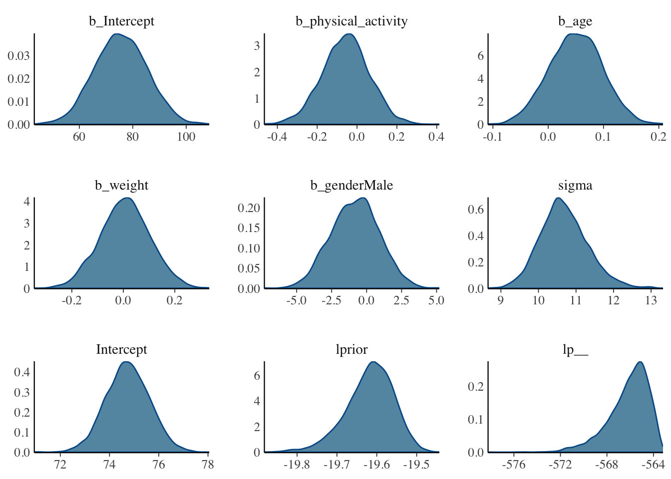
Density Plots: Shows the posterior distributions of the parameters.
Interpretation: These should be smooth and unimodal. Multiple peaks might indicate issues with convergence or that the model has not properly identified the posterior distribution.
# Density Plots (Posterior distributions)mcmc_dens(model) +yaxis_text(TRUE)
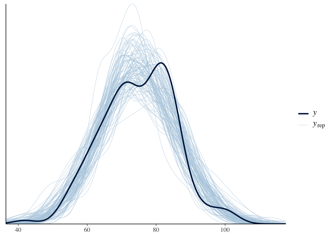
Density Overlay Plot: Compares the density of the observed data to the density of the data generated by the model.
Interpretation: The observed data (solid line) should ideally lie within the range of the simulated data (light blue lines). If the observed data fall outside this range, it may indicate that the model does not fit the data well.