Measuring Perceptions of the Hyperloop
Project Description
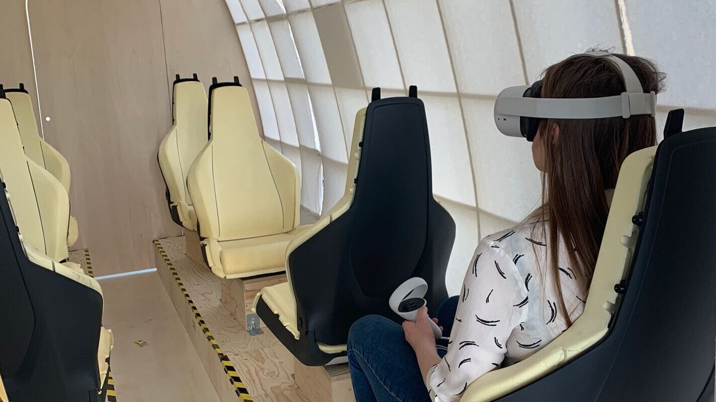
My primary research objective at Hardt Hyperloop was to investigate user perceptions of a simulated hyperloop trip. The company aimed to determine the appropriate dimensions of the hyperloop capsule before investing extensively in materials. However, since the company had not yet developed a hyperloop accessible to the public, predicting how people would feel inside the capsule was challenging. To address this, our team designed a real-life hyperloop experience—a wooden mock-up capsule equipped with seating and accompanied by a VR headset to illustrate the remaining characteristics of the hyperloop interior.
We recruited residents in Groningen to participate in the VR simulation and complete questionnaires. Four main constructs—technology acceptance, perceived safety, perceived comfort, and claustrophobia—were identified for latent class analysis. This model will be instrumental in classifying users in future simulated hyperloop studies.
The dataframe named survey_data contains columns: tech_acceptance, perceived_safety, perceived_comfort, and claustrophobia. Unfortunately, due to privacy laws, I cannot share the data on this platform. I can only provide my code for analyzing the survey data collected at Hardt Hyperloop.
This analysis includes the code for building reliability tests, an LCA model, item structures, and a MMR model.
1. Install Packages
library(poLCA)
library(ggplot2)
library(reshape2)
2. Testing Reliability
survey_data <- read.csv("survey_data.csv")

# Compute Cronbach's alpha for each construct
alpha(survey_data[, c("tech_acceptance_item1", "tech_acceptance_item2", "tech_acceptance_item3", "tech_acceptance_item4", "tech_acceptance_item5", "tech_acceptance_item6", "tech_acceptance_item7", "tech_acceptance_item8", "tech_acceptance_item9", "tech_acceptance_item10")], check.keys=TRUE)
alpha(survey_data[, c("perceived_safety_item1", "perceived_safety_item2", "perceived_safety_item3", "perceived_safety_item4", "perceived_safety_item5")], check.keys=TRUE)
alpha(survey_data[, c("perceived_comfort_item1", "perceived_comfort_item2", "perceived_comfort_item3", "perceived_comfort_item4", "perceived_comfort_item5")], check.keys=TRUE)
alpha(survey_data[, c("claustrophobia_item1", "claustrophobia_item2", "claustrophobia_item3", "claustrophobia_item4")], check.keys=TRUE)
3. Latent-Class Analysis
my_classes <- cbind(tech_acceptance, perceived_safety, perceived_comfort, claustrophobia) ~ 1

survey_data$class <- my_classes$predclass
head(survey_data)
Model Selection
aic_values <- numeric()
bic_values <- numeric()
models <- list()

# Fit LCA models with 1 to 5 classes
for (k in 1:4) {
  lca_model <- poLCA(f, data = survey_data, nclass = k, maxiter = 1000, verbose = FALSE)
  aic_values[k] <- lca_model$aic
  bic_values[k] <- lca_model$bic
  models[[k]] <- lca_model
}

# Combine AIC and BIC values into a new data frame
model_comparison <- data.frame(
  Classes = 1:5,
  AIC = aic_values,
  BIC = bic_values
)

# Simply look for the lowest AIC and BIC
print(model_comparison)
AIC and BIC Plots
model_comparison_melt <- melt(model_comparison, id.vars = "Classes", variable.name = "Metric", value.name = "Value")

ggplot(model_comparison_melt, aes(x = Classes, y = Value, color = Metric)) +
  geom_line() +
  geom_point() +
  theme_minimal() +
  labs(title = "Model Comparison using AIC and BIC",
       x = "Number of Classes",
       y = "Value",
       color = "Metric")
4. Plotting Item Structures
ggplot(survey_data, aes(x = factor(class))) +
  geom_bar(fill = "blue", alpha = 0.7) +
  theme_minimal() +
  labs(title = "Latent Class Memberships",
       x = "Class",
       y = "Count")

# Class-specific item probabilities
item_probs <- lca_model$probs

# Convert to a new data frame for plotting
item_probs_df <- do.call(rbind, lapply(seq_along(item_probs), function(i) {
  item <- names(item_probs)[i]
  probs <- item_probs[[i]]
  data.frame(Class = rep(seq_along(probs), each = nrow(probs)),
             Item = item,
             Category = rep(1:nrow(probs), times = length(probs)),
             Probability = as.vector(probs))
}))

# Plot item profiles
ggplot(item_probs_df, aes(x = Category, y = Probability, fill = factor(Class))) +
  geom_bar(stat = "identity", position = position_dodge()) +
  facet_wrap(~Item, scales = "free_x") +
  theme_minimal() +
  labs(title = "Item Profiles for Latent Classes",
       x = "Category",
       y = "Probability",
       fill = "Class")
5. Multivariate Multiple Regression
# Multivariate multiple regression model
mul_model <- lm(cbind(tech_acceptance, perceived_safety, perceived_comfort, claustrophobia) ~ age + gender, data = survey_data)

# Calculate VIF
vif(mul_model)
Plotting
# Extract coefficients
coefficients <- summary(mmr_model)$coefficients

# Reshape data
coef_df <- data.frame(Variable = rownames(coefficients[[1]]), coefficients)
coef_df <- melt(coef_df, id.vars = "Variable", variable.name = "Outcome", value.name = "Coefficient")

# Plot coefficents
ggplot(coef_df, aes(x = Variable, y = Coefficient, fill = Outcome)) +
  geom_bar(stat = "identity", position = position_dodge()) +
  theme_minimal() +
  labs(title = "Multivariate Multiple Regression Coefficients",
       x = "Predictors",
       y = "Coefficient",
       fill = "Outcome Variables") +
  coord_flip()

# Plot Residuals vs Fitted values for each dependent variable

# Tech Acceptance
plot(mmr_model$fitted.values[, 1], mmr_model$residuals[, 1], main = "Residuals vs Fitted (Tech Acceptance)", xlab = "Fitted Values", ylab = "Residuals")
abline(h = 0, col = "red")

# Perceived Safety
plot(mmr_model$fitted.values[, 2], mmr_model$residuals[, 2], main = "Residuals vs Fitted (Perceived Safety)", xlab = "Fitted Values", ylab = "Residuals")
abline(h = 0, col = "red")

# Perceived Comfort
plot(mmr_model$fitted.values[, 3], mmr_model$residuals[, 3], main = "Residuals vs Fitted (Perceived Comfort)", xlab = "Fitted Values", ylab = "Residuals")
abline(h = 0, col = "red")

# Claustrophobia
plot(mmr_model$fitted.values[, 4], mmr_model$residuals[, 4], main = "Residuals vs Fitted (Claustrophobia)", xlab = "Fitted Values", ylab = "Residuals")
abline(h = 0, col = "red")