Fear Not!

If you’re new to RStudio, you’ve come to the right place. Beyond my advanced projects, I’ve created this beginner-friendly page to share some basic computations. Whether you’re an employer or a colleague visiting, I’m delighted to have your interest.

We all have our first “sense of horror” moment when we first encounter RStudio. For me, it was during my first year in a biostatistics class with my teacher, Tessa. She had us working on projects using RStudio during class, and those initial weeks were chaotic. We were all frustrated and terrified by what appeared on our screens—scary red errors seemed to pop up every second, and we felt like we were making no progress at all. However, Tessa remained by our side. She dedicated the beginning of every class to addressing the typical errors we encountered, guiding us toward smart tactics and helpful online resources.

By the end of the semester, our perception of RStudio had completely changed. Tessa helped us realize that it wasn’t some dark abyss from which no student returns; it was a powerful tool that made statistics easier to compute. We bid farewell to the daunting equations we were accustomed to and began computing statistical techniques at a rapid pace. To this day, every one of my classmates continues to use RStudio with excitement. This software is truly your best friend if you use it wisely.

Learning R

1. Asking for Help

2. Packages

3. Reading Data

4. Tidying Data

5. Functions

6. Data Visualization

1. Asking for Help

Most experts mention asking for help at the end of their tutorials, but I believe it deserves to be first. Learning R involves seeking a lot of assistance, and there are countless online resources available to answer your questions. Below are some of my favorite resources:

• The Help Center in RStudio: Located in the bottom right pane of your window, the Help Center provides detailed explanations of each command in R. You can learn about the purpose of each function, as well as their sub-commands and properties. You can also type any command with the ? symbol in front of it and it will direct you to the same window (e.g., ?plot()).

• The R Project Website: Provides comprehensive documentation and manuals.

• RStudio Community: An active forum where you can ask questions.

• R-Bloggers: A resource for tutorials, tips, and tricks from the R community.

• YouTube: Useful tutorials for visual learners.

• Reddit: A community where everyone deals with problems using R. Visit Reddit to view a wide range of questions and answers from people around the globe.

• Generative AI: An easy tool that can pick out the flaw in your code and guide you toward a solution. However, I recommend you use with caution, as AI can occasionally produce unreliable solutions to your code.

By leveraging these resources, you can make your learning journey with R more efficient and less daunting.

2. Packages

R packages are collections of functions, data, and documentation that extend the capabilities of base R, making it easier and more efficient to perform a wide range of tasks.

• Simplify Complex Tasks

• Improve Data Analysis

• Improve Data Visualization

• Streamline Workflow

Here are some of the most common or important packages in R used in the social sciences:

• ggplot2: Customizable plots

• dplyr: Data manipulation

• tidyr: Cleaning data

• stringr: String manipulation

• lubridate: Dates and times

• psych: Psychometrics and psychological research

• lme4: Linear and generalized linear mixed-effects models

• afex: Factorial analysis

• bayesplotorbrms: Bayesian statistics

The tidyverse is a collection of R packages designed for data science. The core packages included in tidyverse are ggplot2, tidyr, readr, dplyr, andstringr. You can also download these packages separately.

3. Reading data.

1. Loading a file

You can find your data either using the file.choose() function or by clicking on Files in the bottom right window. Make sure to save your new data in your local Environment in the top right window.

2. CSV Files

The most common format for data files is CSV (Comma-Separated Values). The readr package from the tidyverse provides functions to read CSV files efficiently.

library(tidyverse)

── Attaching core tidyverse packages ──────────────────────── tidyverse 2.0.0 ──
✔ dplyr     1.1.4     ✔ readr     2.1.5
✔ forcats   1.0.0     ✔ stringr   1.5.1
✔ ggplot2   3.5.1     ✔ tibble    3.2.1
✔ lubridate 1.9.3     ✔ tidyr     1.3.1
✔ purrr     1.0.2     
── Conflicts ────────────────────────────────────────── tidyverse_conflicts() ──
✖ dplyr::filter() masks stats::filter()
✖ dplyr::lag()    masks stats::lag()
ℹ Use the conflicted package (<http://conflicted.r-lib.org/>) to force all conflicts to become errors

# Read CSV file
data <- read.csv("exercise_data.csv")

3. Excel Files

library(readxl)

# Read the first sheet
data <- read_excel("/Users/owencallahan/Downloads/Fitness.xlsx")

# Read a specific sheet by name
data_sheet <- read_excel("/Users/owencallahan/Downloads/Fitness.xlsx", sheet = "Sheet1")

# Read a specific sheet by index
data_index <- read_excel("/Users/owencallahan/Downloads/Fitness.xlsx", sheet = 1)

4. Writing Data

data <- c(1,2,3,4)
write.csv(data, "my_data.csv")

4. Tidying Data

Tidying data is an essential part of data analysis in R, making your data easier to work with and analyze. We’ll use the tidyverse suite of packages, which includes dplyr, tidyr, and readr among others. Below is a step-by-step tutorial with code examples to demonstrate how to tidy data in R.

1. Structuring Data formats.

Pivoting longer:

wide_data <- tibble(
  id = 1:3,
  age = c(25, 30, 35),
  height = c(175, 180, 165),
  weight = c(70, 80, 65)
)

# Convert to long format
long_data <- wide_data %>%
  pivot_longer(cols = c(age, height, weight), names_to = "measure", values_to = "value")

print(long_data)

# A tibble: 9 × 3
     id measure value
  <int> <chr>   <dbl>
1     1 age        25
2     1 height    175
3     1 weight     70
4     2 age        30
5     2 height    180
6     2 weight     80
7     3 age        35
8     3 height    165
9     3 weight     65

Pivoting wider:

# Convert back to wide format
wide_again <- long_data %>%
  pivot_wider(names_from = measure, values_from = value)

print(wide_again)

# A tibble: 3 × 4
     id   age height weight
  <int> <dbl>  <dbl>  <dbl>
1     1    25    175     70
2     2    30    180     80
3     3    35    165     65

Separate columns:

data <- tibble(
  name = c("John_Doe", "Jane_Smith", "Alice_Johnson")
)

# Separate into first and last names
separated_data <- data %>%
  separate(name, into = c("first_name", "last_name"), sep = "_")

print(separated_data)

# A tibble: 3 × 2
  first_name last_name
  <chr>      <chr>    
1 John       Doe      
2 Jane       Smith    
3 Alice      Johnson  

Unite columns:

united_data <- separated_data %>%
  unite("full_name", first_name, last_name, sep = " ")

2. Select, filter, mutate, and summarize data.

Selecting Columns

selected_data <- mtcars %>%
  select(cyl, gear)

head(selected_data)

                  cyl gear
Mazda RX4           6    4
Mazda RX4 Wag       6    4
Datsun 710          4    4
Hornet 4 Drive      6    3
Hornet Sportabout   8    3
Valiant             6    3

Filtering Rows

filtered_data <- mtcars %>%
  filter(gear < 4)

head(filtered_data)

                   mpg cyl  disp  hp drat    wt  qsec vs am gear carb
Hornet 4 Drive    21.4   6 258.0 110 3.08 3.215 19.44  1  0    3    1
Hornet Sportabout 18.7   8 360.0 175 3.15 3.440 17.02  0  0    3    2
Valiant           18.1   6 225.0 105 2.76 3.460 20.22  1  0    3    1
Duster 360        14.3   8 360.0 245 3.21 3.570 15.84  0  0    3    4
Merc 450SE        16.4   8 275.8 180 3.07 4.070 17.40  0  0    3    3
Merc 450SL        17.3   8 275.8 180 3.07 3.730 17.60  0  0    3    3

Mutating Columns

mutated_data <- mtcars %>%
  mutate(speed.scale = qsec/wt)

head(mutated_data %>%
        select(speed.scale))

                  speed.scale
Mazda RX4            6.282443
Mazda RX4 Wag        5.920000
Datsun 710           8.021552
Hornet 4 Drive       6.046656
Hornet Sportabout    4.947674
Valiant              5.843931

Summarizing Data

summary_data <- mtcars %>%
  group_by(gear) %>%
  summarize(
    average_wt = mean(wt),
    count = n()
  )

print(summary_data)

# A tibble: 3 × 3
   gear average_wt count
  <dbl>      <dbl> <int>
1     3       3.89    15
2     4       2.62    12
3     5       2.63     5

3. Handle missing values.

# Identify missing values
missing_data <- mtcars %>%
  filter(is.na(wt))

# Remove rows with missing values
cleaned_data <- data %>%
  drop_na()

# Replace missing values with a specific value
filled_data <- data %>%
  replace_na(list(height = 170, weight = 70))

4. Combine datasets.

data1 <- tibble(
  id = 1:3,
  name = c("John", "Jane", "Alice")
)

data2 <- tibble(
  id = 1:3,
  score = c(85, 90, 78)
)

# Inner join
joined_data <- data1 %>%
  inner_join(data2, by = "id")

print(joined_data)

# A tibble: 3 × 3
     id name  score
  <int> <chr> <dbl>
1     1 John     85
2     2 Jane     90
3     3 Alice    78

5. Functions

When I learned how to create my own functions, I felt like the creative side of R expanded beyond my expectations. I could tailor a command to address exactly what I needed to perform on a given set of data.

1. Building Functions

The function() command is a fundamental building block in R, enabling users to create their own functions. This is crucial for both simplifying repetitive tasks and organizing code in a clean, efficient manner. Here’s what the function() command can do for new learners using R:

• Encapsulate Repetitive Tasks

  • Creating functions allows you to encapsulate repetitive code into reusable blocks. This reduces redundancy and makes your scripts more concise and readable. For example, if you frequently perform the same data transformation, you can write a function for it and call it whenever needed.

• Organize Code

  • Functions help in organizing code logically. By breaking down complex procedures into smaller, manageable functions, you make your code more modular and easier to debug and maintain.

• Improve Readability

  • Using functions can significantly enhance the readability of your code. Descriptive function names and clear parameter definitions help others (and your future self) understand the purpose and usage of the code more quickly.

• Parameterization

  • Functions allow you to use parameters to make your code more flexible. Instead of hard-coding values, you can pass different arguments to your functions, making them adaptable to various inputs and scenarios.

• Enhance Reproducibility

  • Functions contribute to reproducibility in your analyses. By encapsulating specific tasks, you ensure that the same operations can be repeated with different data or settings, leading to consistent results.

• Promote Code Reuse

  • Once you write a function, you can reuse it across different projects. This saves time and effort, as you don’t need to rewrite the same code for similar tasks.

Example of Using function() in R

# Define a function to calculate the mean of a numeric vector
calculate_mean <- function(numbers) {
  mean_value <- mean(numbers)
  return(mean_value)
}

# Use the function with a numeric vector
sample_data <- c(4, 8, 15, 16, 23, 42)
average <- calculate_mean(sample_data)
print(average)

[1] 18

2. Correlation Analysis

Correlation measures the strength and direction of the relationship between two variables.

# Correlation matrix
cor_matrix <- cor(mtcars)
print(cor_matrix)

            mpg        cyl       disp         hp        drat         wt
mpg   1.0000000 -0.8521620 -0.8475514 -0.7761684  0.68117191 -0.8676594
cyl  -0.8521620  1.0000000  0.9020329  0.8324475 -0.69993811  0.7824958
disp -0.8475514  0.9020329  1.0000000  0.7909486 -0.71021393  0.8879799
hp   -0.7761684  0.8324475  0.7909486  1.0000000 -0.44875912  0.6587479
drat  0.6811719 -0.6999381 -0.7102139 -0.4487591  1.00000000 -0.7124406
wt   -0.8676594  0.7824958  0.8879799  0.6587479 -0.71244065  1.0000000
qsec  0.4186840 -0.5912421 -0.4336979 -0.7082234  0.09120476 -0.1747159
vs    0.6640389 -0.8108118 -0.7104159 -0.7230967  0.44027846 -0.5549157
am    0.5998324 -0.5226070 -0.5912270 -0.2432043  0.71271113 -0.6924953
gear  0.4802848 -0.4926866 -0.5555692 -0.1257043  0.69961013 -0.5832870
carb -0.5509251  0.5269883  0.3949769  0.7498125 -0.09078980  0.4276059
            qsec         vs          am       gear        carb
mpg   0.41868403  0.6640389  0.59983243  0.4802848 -0.55092507
cyl  -0.59124207 -0.8108118 -0.52260705 -0.4926866  0.52698829
disp -0.43369788 -0.7104159 -0.59122704 -0.5555692  0.39497686
hp   -0.70822339 -0.7230967 -0.24320426 -0.1257043  0.74981247
drat  0.09120476  0.4402785  0.71271113  0.6996101 -0.09078980
wt   -0.17471588 -0.5549157 -0.69249526 -0.5832870  0.42760594
qsec  1.00000000  0.7445354 -0.22986086 -0.2126822 -0.65624923
vs    0.74453544  1.0000000  0.16834512  0.2060233 -0.56960714
am   -0.22986086  0.1683451  1.00000000  0.7940588  0.05753435
gear -0.21268223  0.2060233  0.79405876  1.0000000  0.27407284
carb -0.65624923 -0.5696071  0.05753435  0.2740728  1.00000000

# Correlation between two variables
cor(mtcars$mpg, mtcars$hp)

[1] -0.7761684

3. Linear Regression

Linear regression models the relationship between a dependent variable and one or more independent variables.

# Simple linear regression
model <- lm(mpg ~ hp, data = mtcars)
summary(model)

Call:
lm(formula = mpg ~ hp, data = mtcars)

Residuals:
    Min      1Q  Median      3Q     Max 
-5.7121 -2.1122 -0.8854  1.5819  8.2360 

Coefficients:
            Estimate Std. Error t value Pr(>|t|)    
(Intercept) 30.09886    1.63392  18.421  < 2e-16 ***
hp          -0.06823    0.01012  -6.742 1.79e-07 ***
---
Signif. codes:  0 '***' 0.001 '**' 0.01 '*' 0.05 '.' 0.1 ' ' 1

Residual standard error: 3.863 on 30 degrees of freedom
Multiple R-squared:  0.6024,    Adjusted R-squared:  0.5892 
F-statistic: 45.46 on 1 and 30 DF,  p-value: 1.788e-07

# Multiple linear regression
model2 <- lm(mpg ~ hp + wt, data = mtcars)
summary(model2)

Call:
lm(formula = mpg ~ hp + wt, data = mtcars)

Residuals:
   Min     1Q Median     3Q    Max 
-3.941 -1.600 -0.182  1.050  5.854 

Coefficients:
            Estimate Std. Error t value Pr(>|t|)    
(Intercept) 37.22727    1.59879  23.285  < 2e-16 ***
hp          -0.03177    0.00903  -3.519  0.00145 ** 
wt          -3.87783    0.63273  -6.129 1.12e-06 ***
---
Signif. codes:  0 '***' 0.001 '**' 0.01 '*' 0.05 '.' 0.1 ' ' 1

Residual standard error: 2.593 on 29 degrees of freedom
Multiple R-squared:  0.8268,    Adjusted R-squared:  0.8148 
F-statistic: 69.21 on 2 and 29 DF,  p-value: 9.109e-12

4. ANOVA (Analysis of Variance)

ANOVA tests the difference in means among groups.

# One-way ANOVA
anova_model <- aov(mpg ~ as.factor(cyl), data = mtcars)
summary(anova_model)

               Df Sum Sq Mean Sq F value   Pr(>F)    
as.factor(cyl)  2  824.8   412.4    39.7 4.98e-09 ***
Residuals      29  301.3    10.4                     
---
Signif. codes:  0 '***' 0.001 '**' 0.01 '*' 0.05 '.' 0.1 ' ' 1

# Two-way ANOVA
anova_model2 <- aov(mpg ~ as.factor(cyl) + as.factor(gear), data = mtcars)
summary(anova_model2)

                Df Sum Sq Mean Sq F value   Pr(>F)    
as.factor(cyl)   2  824.8   412.4   38.00 1.41e-08 ***
as.factor(gear)  2    8.3     4.1    0.38    0.687    
Residuals       27  293.0    10.9                     
---
Signif. codes:  0 '***' 0.001 '**' 0.01 '*' 0.05 '.' 0.1 ' ' 1

5. T-tests

T-tests compare the means of two groups.

# One-sample t-test
t.test(mtcars$mpg, mu = 20)

    One Sample t-test

data:  mtcars$mpg
t = 0.08506, df = 31, p-value = 0.9328
alternative hypothesis: true mean is not equal to 20
95 percent confidence interval:
 17.91768 22.26357
sample estimates:
mean of x 
 20.09062 

# Two-sample t-test
t.test(mpg ~ as.factor(am), data = mtcars)

    Welch Two Sample t-test

data:  mpg by as.factor(am)
t = -3.7671, df = 18.332, p-value = 0.001374
alternative hypothesis: true difference in means between group 0 and group 1 is not equal to 0
95 percent confidence interval:
 -11.280194  -3.209684
sample estimates:
mean in group 0 mean in group 1 
       17.14737        24.39231 

6. Chi-Square Test

Chi-square tests are used for categorical data to test relationships between variables.

# Create a contingency table
table_data <- table(mtcars$cyl, mtcars$gear)

# Chi-square test
chisq.test(table_data)

Warning in chisq.test(table_data): Chi-squared approximation may be incorrect

    Pearson's Chi-squared test

data:  table_data
X-squared = 18.036, df = 4, p-value = 0.001214

7. Principal Component Analysis (PCA)

PCA reduces the dimensionality of the data while preserving as much variance as possible. An excellent tutorial on PCA can be found by clicking this link: https://www.youtube.com/watch?

# Perform PCA
pca_result <- prcomp(mtcars, scale. = TRUE)

# Summary of PCA
summary(pca_result)

Importance of components:
                          PC1    PC2     PC3     PC4     PC5     PC6    PC7
Standard deviation     2.5707 1.6280 0.79196 0.51923 0.47271 0.46000 0.3678
Proportion of Variance 0.6008 0.2409 0.05702 0.02451 0.02031 0.01924 0.0123
Cumulative Proportion  0.6008 0.8417 0.89873 0.92324 0.94356 0.96279 0.9751
                           PC8    PC9    PC10   PC11
Standard deviation     0.35057 0.2776 0.22811 0.1485
Proportion of Variance 0.01117 0.0070 0.00473 0.0020
Cumulative Proportion  0.98626 0.9933 0.99800 1.0000

8. K-Means Clustering

K-means clustering groups data into k clusters.

# Perform K-means clustering on the mtcars dataset
set.seed(123)
kmeans_result <- kmeans(mtcars[, c("mpg", "hp")], centers = 3)

# Add cluster results to the original mtcars data
mtcars$cluster <- as.factor(kmeans_result$cluster)

# Print the first few rows to check the results
head(mtcars)

                   mpg cyl disp  hp drat    wt  qsec vs am gear carb cluster
Mazda RX4         21.0   6  160 110 3.90 2.620 16.46  0  1    4    4       3
Mazda RX4 Wag     21.0   6  160 110 3.90 2.875 17.02  0  1    4    4       3
Datsun 710        22.8   4  108  93 3.85 2.320 18.61  1  1    4    1       3
Hornet 4 Drive    21.4   6  258 110 3.08 3.215 19.44  1  0    3    1       3
Hornet Sportabout 18.7   8  360 175 3.15 3.440 17.02  0  0    3    2       2
Valiant           18.1   6  225 105 2.76 3.460 20.22  1  0    3    1       3

9. Logistic Regression

Logistic regression models the probability of a binary outcome.

# Logistic regression
logit_model <- glm(am ~ hp + wt, data = mtcars, family = binomial)
summary(logit_model)

Call:
glm(formula = am ~ hp + wt, family = binomial, data = mtcars)

Coefficients:
            Estimate Std. Error z value Pr(>|z|)   
(Intercept) 18.86630    7.44356   2.535  0.01126 * 
hp           0.03626    0.01773   2.044  0.04091 * 
wt          -8.08348    3.06868  -2.634  0.00843 **
---
Signif. codes:  0 '***' 0.001 '**' 0.01 '*' 0.05 '.' 0.1 ' ' 1

(Dispersion parameter for binomial family taken to be 1)

    Null deviance: 43.230  on 31  degrees of freedom
Residual deviance: 10.059  on 29  degrees of freedom
AIC: 16.059

Number of Fisher Scoring iterations: 8

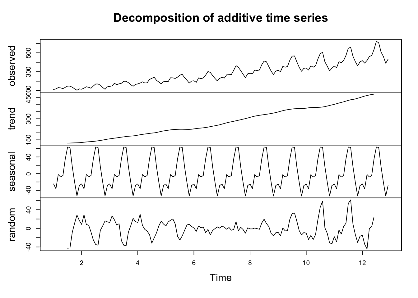
10. Time Series Analysis

# Decomposition

# Sample time series data
ts_data <- ts(AirPassengers, frequency = 12)

# Decompose the time series
decomposed <- decompose(ts_data)
plot(decomposed)

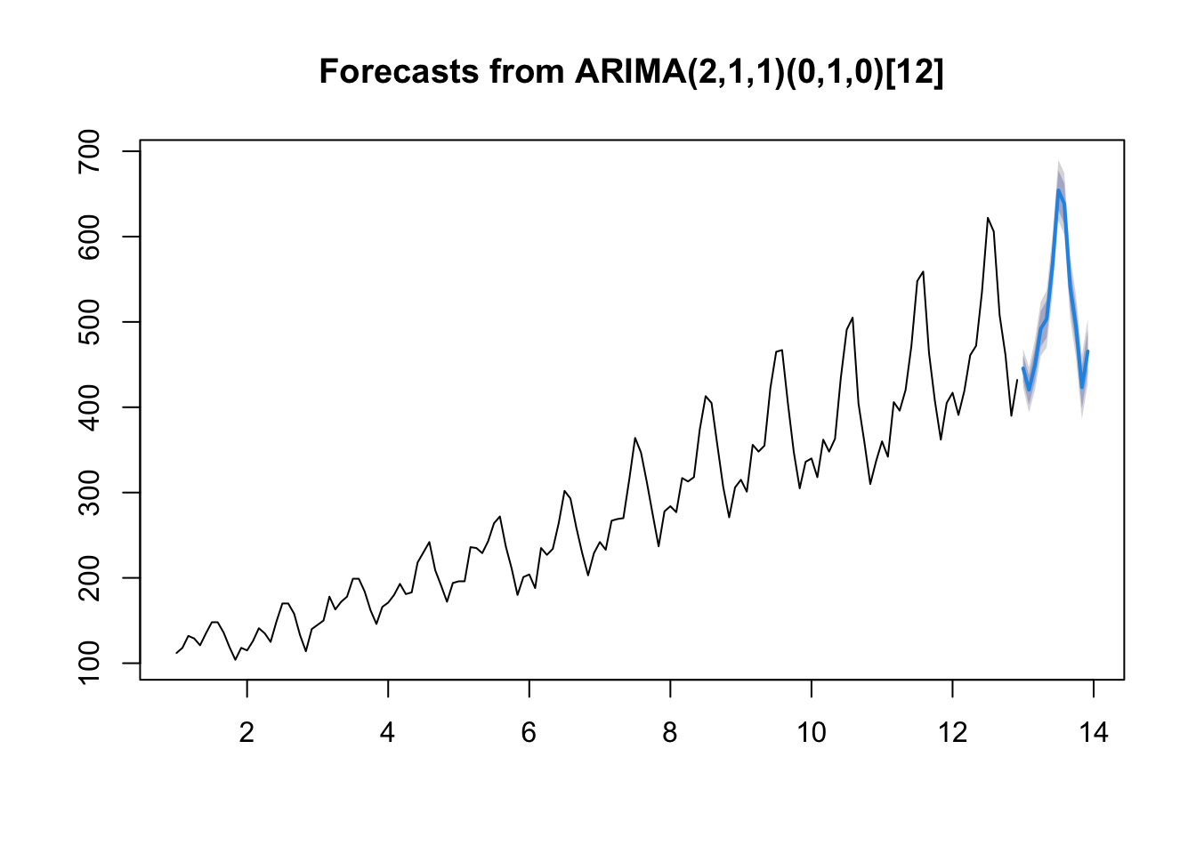
# Forecasting

# Install and load the forecast package
library(forecast)

Registered S3 method overwritten by 'quantmod':
  method            from
  as.zoo.data.frame zoo 

# Fit an ARIMA model
fit <- auto.arima(ts_data)
forecasted <- forecast(fit, h = 12)
plot(forecasted)

6. Data Visualization

Let’s explore one of my favorite, and also one of the most essential packages in R, ggplot2.

1. Installation and Loading

First, you need to install and load the ggplot2 package:

options(repos = c(CRAN = "https://cloud.r-project.org"))
install.packages("ggplot2")

The downloaded binary packages are in
    /var/folders/k3/v39j6g_x4bv7mv_xq03986d00000gn/T//RtmpQAa8X7/downloaded_packages

library(ggplot2)

2. Basic Components

ggplot2 follows the grammar of graphics, which means you build plots layer by layer. The essential components are:

• Data: The dataset you’re plotting.

• Aesthetics (aes): The mapping of variables to visual properties like x and y coordinates, colors, sizes, etc.

• Geometries (geom): The type of plot you want to create (e.g., points, lines, bars).

• Facets: Subplots based on the values of one or more variables.

• Scales: Control how data values are mapped to visual properties.

• Coordinate Systems: Control the coordinate space.

• Themes: Control the appearance of the plot.

3. Basic Plot Types

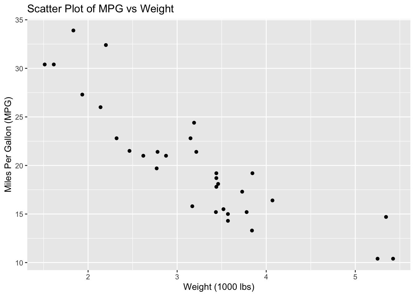
Scatter Plot

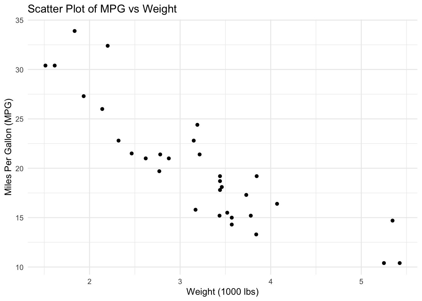
# Load example data
data(mtcars)

# Create a scatter plot
ggplot(data = mtcars, aes(x = wt, y = mpg)) +
  geom_point() +
  labs(title = "Scatter Plot of MPG vs Weight",
       x = "Weight (1000 lbs)",
       y = "Miles Per Gallon (MPG)")

Line Plot

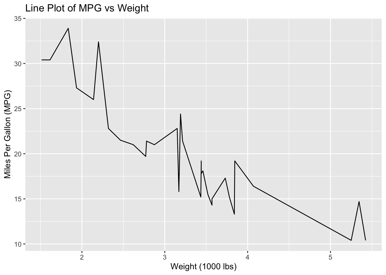
# Create a line plot
ggplot(data = mtcars, aes(x = wt, y = mpg)) +
  geom_line() +
  labs(title = "Line Plot of MPG vs Weight",
       x = "Weight (1000 lbs)",
       y = "Miles Per Gallon (MPG)")

Bar Plot

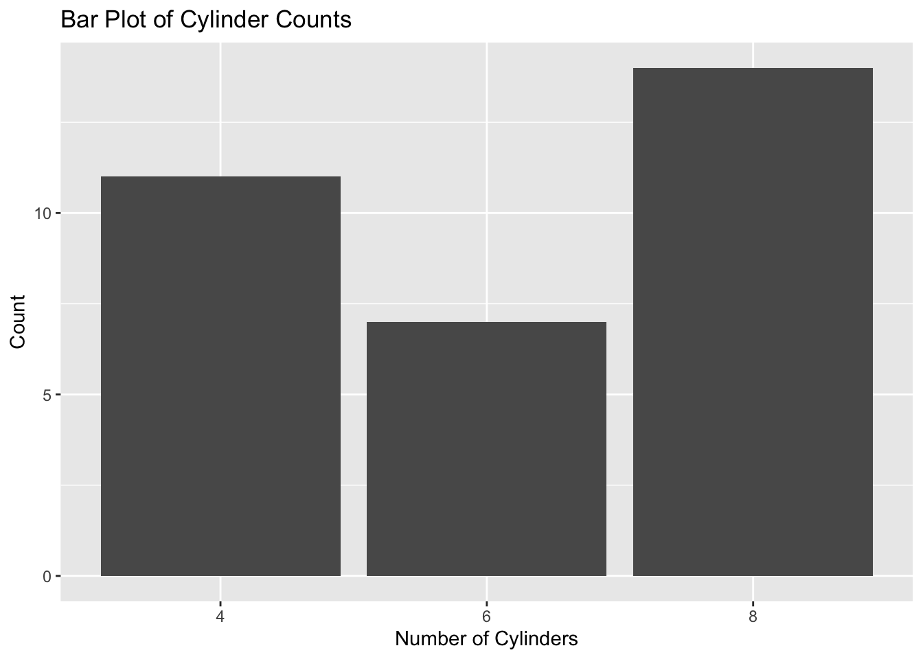
# Create a bar plot
ggplot(data = mtcars, aes(x = factor(cyl))) +
  geom_bar() +
  labs(title = "Bar Plot of Cylinder Counts",
       x = "Number of Cylinders",
       y = "Count")

Histogram

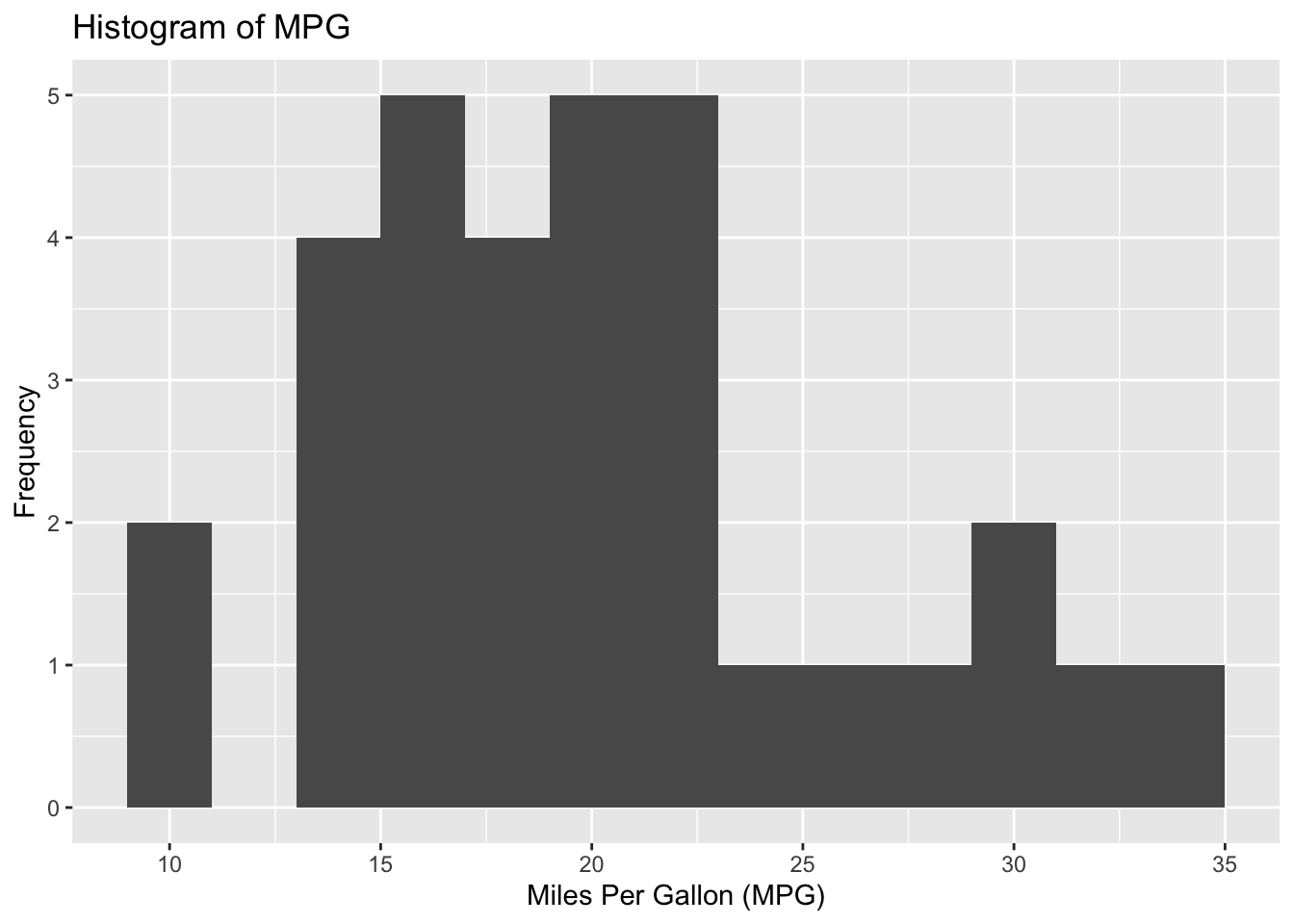
# Create a histogram
ggplot(data = mtcars, aes(x = mpg)) +
  geom_histogram(binwidth = 2) +
  labs(title = "Histogram of MPG",
       x = "Miles Per Gallon (MPG)",
       y = "Frequency")

Box Plot

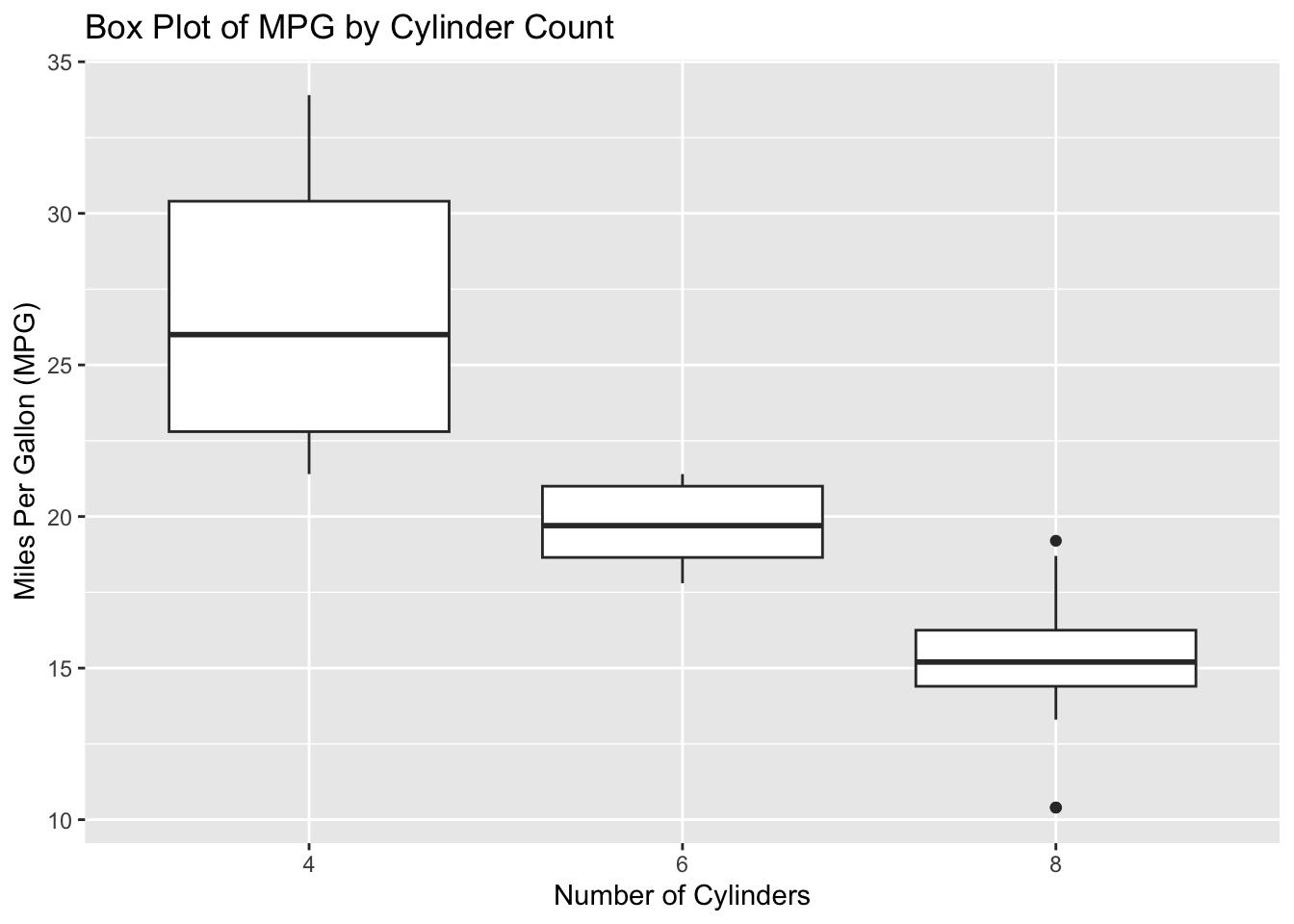
# Create a box plot
ggplot(data = mtcars, aes(x = factor(cyl), y = mpg)) +
  geom_boxplot() +
  labs(title = "Box Plot of MPG by Cylinder Count",
       x = "Number of Cylinders",
       y = "Miles Per Gallon (MPG)")

4. Customizing Plots

Adding Colors

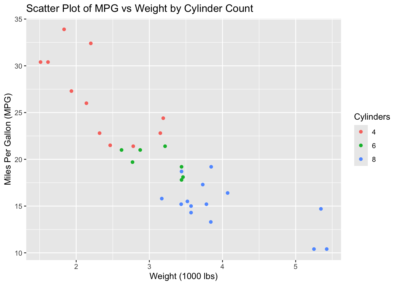
# Scatter plot with color
ggplot(data = mtcars, aes(x = wt, y = mpg, color = factor(cyl))) +
  geom_point() +
  labs(title = "Scatter Plot of MPG vs Weight by Cylinder Count",
       x = "Weight (1000 lbs)",
       y = "Miles Per Gallon (MPG)",
       color = "Cylinders")

Adding Size

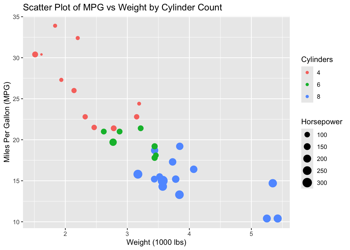
# Scatter plot with color and size
ggplot(data = mtcars, aes(x = wt, y = mpg, color = factor(cyl), size = hp)) +
  geom_point() +
  labs(title = "Scatter Plot of MPG vs Weight by Cylinder Count",
       x = "Weight (1000 lbs)",
       y = "Miles Per Gallon (MPG)",
       color = "Cylinders",
       size = "Horsepower")

Faceting

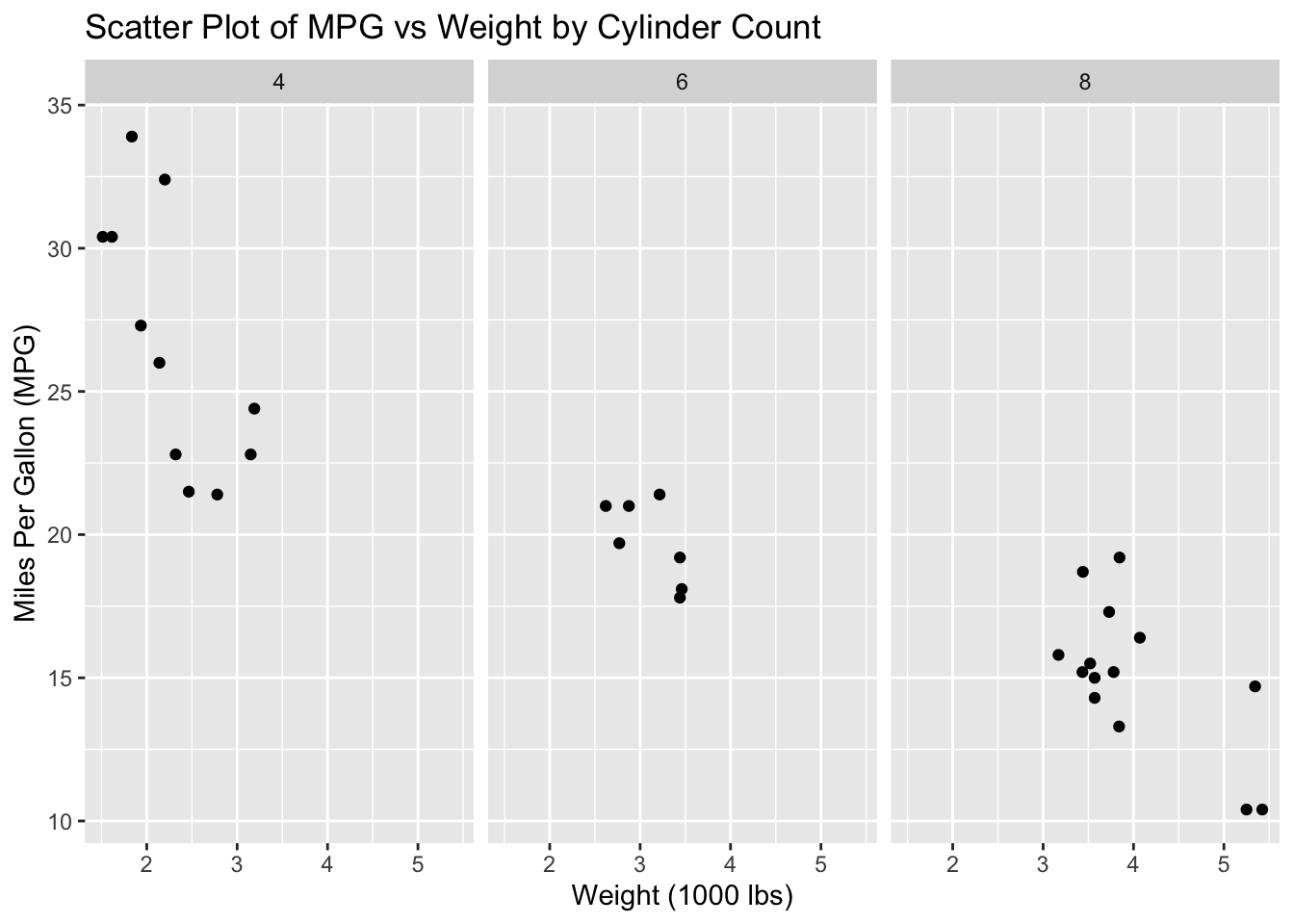
# Faceted scatter plot
ggplot(data = mtcars, aes(x = wt, y = mpg)) +
  geom_point() +
  facet_wrap(~ cyl) +
  labs(title = "Scatter Plot of MPG vs Weight by Cylinder Count",
       x = "Weight (1000 lbs)",
       y = "Miles Per Gallon (MPG)")

Themes

# Scatter plot with theme
ggplot(data = mtcars, aes(x = wt, y = mpg)) +
  geom_point() +
  labs(title = "Scatter Plot of MPG vs Weight",
       x = "Weight (1000 lbs)",
       y = "Miles Per Gallon (MPG)") +
  theme_minimal()