This is a research project I developed during my Master’s Degree in Environmental Psychology. It includes a hierarchical model that explores the cross-level dynamics within communities in the Netherlands.
I am still motivated about executing this project again in a different setting because it addresses contemporary challenges in ethnically heterogeneous neighborhoods and provides an unique approach to understanding social cohesion. It assesses the individual-level, cognitive processes in neighborhood behavior through spatial measurement, which can offer alternative evidence for policymakers’ views toward contextual level action (e.g., developing economically vital cities, demolition, and housing renovation) (Van Kempen & Bolt, 2009). By bridging the gap between individual-level processes and neighborhood dynamics, this research has the potential to inform policy interventions and community development initiatives.
Outcome Variable
boundary: combined value of perceived neighborhood scale and perceived trust in neighbors
Demographics:
age: Normally distributed continuous variable.
education: Dichotomous variable
income: Ordinal variable from 1 to 5.
ethnicity: Categorical variable sampled from four categories “A”, “B”, “C”, and “D”.
length_res: Normally distributed continuous variable for length of residency.
Linking to GEOS 3.11.0, GDAL 3.5.3, PROJ 9.1.0; sf_use_s2() is TRUE
library(ggplot2)library(dplyr)
Attaching package: 'dplyr'
The following objects are masked from 'package:stats':

    filter, lag
The following objects are masked from 'package:base':

    intersect, setdiff, setequal, union
library(geojsonio)
Registered S3 method overwritten by 'geojsonsf':
  method        from
  print.geojson geojson
Attaching package: 'geojsonio'
The following object is masked from 'package:base':

    pretty
library(sp)library(lme4)
Loading required package: Matrix
library(car)
Loading required package: carData
Attaching package: 'car'
The following object is masked from 'package:dplyr':

    recode
library(ggplot2)# Read the GeoJSON mapping filemap_data <-geojson_read("map_data.geojson", what ="sp")map_sf <-st_as_sf(map_data)# Calculate the area of each drawn boundarymap_sf <- map_sf %>%mutate(area =st_area(geometry))map_sf$area <-as.numeric(map_sf$area)
# Load the survey datasetdata <-read.csv("multilevel_model_data.csv")# Merge datasetsdata$id <-1:nrow(data)data <- data %>%left_join(map_sf %>%select(id, area), by ="id")
2. Exploratory Data Analysis
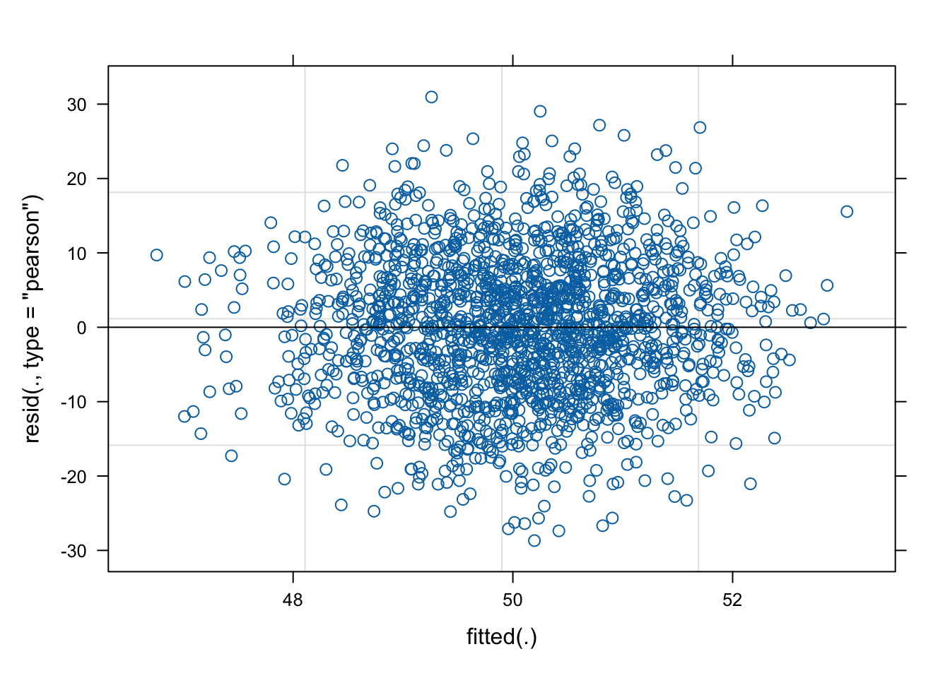
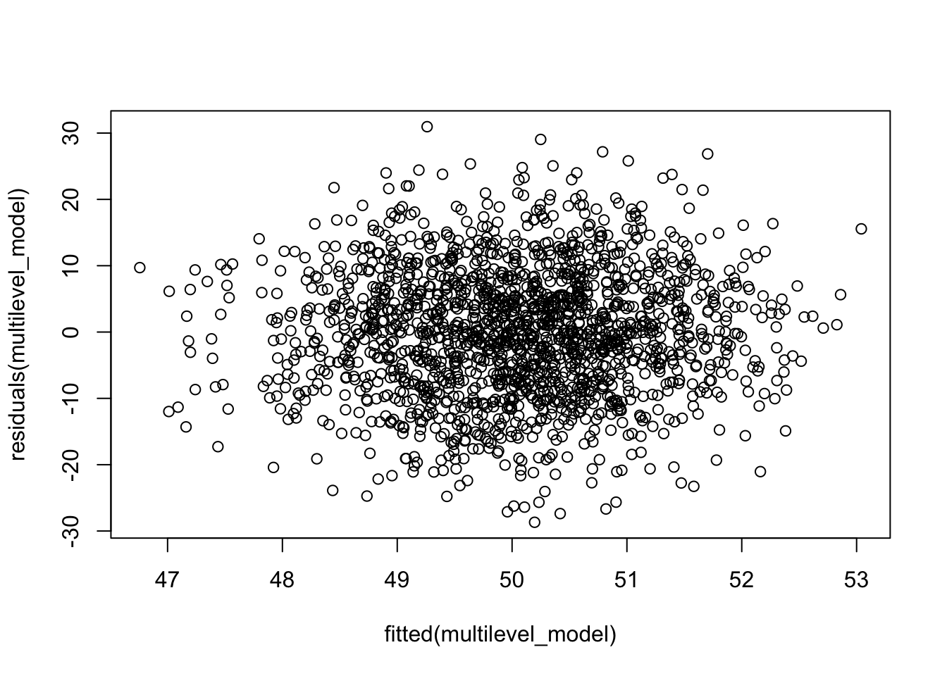
Before I compare the models, let’s take a look at the full model and understand our data a bit better.
# Fit the multilevel modelmultilevel_model <-lmer(boundary ~ age + education + income + ethnicity + length_res + physical_disorder + perceived_collective_efficacy + facilities + names + art + playgrounds + leadership + (1| neighborhood_id), data = data)summary(multilevel_model)
Linear mixed model fit by REML ['lmerMod']
Formula: boundary ~ age + education + income + ethnicity + length_res +
    physical_disorder + perceived_collective_efficacy + facilities +
    names + art + playgrounds + leadership + (1 | neighborhood_id)
   Data: data

REML criterion at convergence: 12877.4

Scaled residuals:
    Min      1Q  Median      3Q     Max
-2.9966 -0.7063  0.0071  0.6710  3.2348

Random effects:
 Groups          Name        Variance Std.Dev.
 neighborhood_id (Intercept)  0.5319  0.7293
 Residual                    91.6096  9.5713
Number of obs: 1750, groups:  neighborhood_id, 25

Fixed effects:
                               Estimate Std. Error t value
(Intercept)                   49.019346   1.575249  31.118
age                           -0.009148   0.015198  -0.602
education                     -0.211335   0.469636  -0.450
income                        -0.425076   0.164823  -2.579
ethnicityB                     0.541790   0.645876   0.839
ethnicityMe                    0.439613   0.651204   0.675
ethnicityW                     0.359890   0.650369   0.553
length_res                    -0.052653   0.076229  -0.691
physical_disorder              0.063064   0.162170   0.389
perceived_collective_efficacy  0.366557   0.232243   1.578
facilities                     0.163935   0.155372   1.055
names                         -0.091896   0.600375  -0.153
art                            0.821966   0.597757   1.375
playgrounds                   -0.077756   0.566788  -0.137
leadership                     0.746840   0.585630   1.275
Correlation matrix not shown by default, as p = 15 > 12.
Use print(x, correlation=TRUE)  or
    vcov(x)        if you need it
After removing variables (age, length_res, names, playgrounds, physical_disorder) , my first adjusted model has one of the lower AIC/BIC, while also aligning with my theoretical framework and hypotheses.
4. Results
# Plot Cooks D estimates with influence plotinfluencePlot(alt_model1, id.n =5)
Warning in plot.window(...): "id.n" is not a graphical parameter
Warning in plot.xy(xy, type, ...): "id.n" is not a graphical parameter
Warning in axis(side = side, at = at, labels = labels, ...): "id.n" is not a
graphical parameter
Warning in axis(side = side, at = at, labels = labels, ...): "id.n" is not a
graphical parameter
Warning in box(...): "id.n" is not a graphical parameter
Warning in title(...): "id.n" is not a graphical parameter
Warning in plot.xy(xy.coords(x, y), type = type, ...): "id.n" is not a
graphical parameter